Optimal Choice - Mathematical Advice for Real Life
Abstract
We discuss how to choose the optimal candidate from a rankable sequence of candidates arriving one by one. The candidates could for example be job applicants, princes, tinder profiles or flats. This choice problem is casted into the context of sequential decision making and is solved using optimal stopping theory. Two R functions are provided to compute optimal selection strategies in two specific instances of the problem. Altogether, the mathematical inclined decision maker is given valuable open-source tools to support prudent real life decision making.
 This work is licensed under a Creative Commons
Attribution-ShareAlike 4.0 International License. The
markdown+Rknitr source code of this blog is available under a GNU General Public
License (GPL v3) license from github.
Introduction
Life is full of choices. The prudent decision maker likes to rationally balance alternatives, assess uncertain outcomes, gather additional information and - when ready - pick the best action. A mathematical approach to such decision making under uncertainty is based on maximizing an adequate utility function subject to the identified stochasticity, e.g., by maximizing expected utility. The ultimate statistical guides to such optimal decision making are the books by DeGroot (1970) and Berger (1985). Influence diagrams are compact representations of decision problems embedded within the graphical modelling toolset of Bayesian networks, see e.g. Jensen and Nielsen (2007).

In this note we consider the very simple – but entertaining – sequential decision problem known as the optimal choice, secretary, marriage, dowry or game of googol problem (Ferguson 1989). Scientific publishing about the optimal choice problem dates back to the 1950’s and 1960’s, but accounts of variations of the problem date back as far as 1613. To illustrate the problem we use the process of finding a real estate property in an overheated housing market as example. Of course, the human resource manager, wooed princess, Johannes Kepler, tinder hustler as well as the mathematical enthusiast (subsets might overlap) should easily be able to adapt terminology to their needs.
The optimal choice problem
The rules of the game are as follows:
- You want to choose exactly one property (say, buy a flat) within a given period of time
- The number of candidate flats available on the market and inspectable in the given time period is assumed to be known. We shall denote this number by \(n\).
- The flats are assumed to be rankable from best (rank 1) to worst (rank \(n\)) without ties.
- The flats can only be inspected sequentially and in some random order.
- After seeing a flat one has to decide whether to pick this flat or not.
- Once a flat is rejected, this choice is permanent and cannot be re-called.
Your objective is to find the best candidate among the \(n\) flats. Less will not work for you, i.e. you have no interest in the 2nd best candidate or any other worse candidate. Furthermore, the decision you have to make at each decision time is to either select the current candidate flat or reject it and inspect futher candidate flats. Which flat to pick thus at each time point is based only on the flat’s relative rank within the set of flats seen up to now. Our goal is to find a strategy s.t. we end up with the best flat, i.e. rank 1, among all of the \(n\) flats. Note that simply looking at all candidates and then picking the best one will not work due to rules 5 and 6.
Mathematical notation
Following Chow et al. (1964) we introduce the following mathematical notation: Let \(x_1,\ldots, x_n\) be a permutation of the integers between 1 and \(n\). At the time we are considering the \(i\)’th candidate in our ordered sequence we have seen the candidates \(1,\ldots,i\). Let \(y_i\), \(y_i \in \{1,\ldots,i\}\), denote the rank of the \(i\)’th candidate among these \(i\) candidates. We call this the relative rank at time \(i\) of the \(i\)’th candidate. Note that the relative rank can be 1 even though a candidates’ overall rank is not 1. This is a consequence of the overall rank being only partially revealed by knowing more of the candidates.
A code example illustrates the concept:
#Generate a sequence of ranks between 1 and n
set.seed(123)
n <- 10L ; x <- sample(1:n,replace=FALSE)

#Function to compute sequential relative ranks, where smallest is best
#Now programmed with Rcpp, which is faster than plain R. Github code
#contains an even faster version relrank_rcpp_novec. Note index start at 0
#in Rcpp.
Rcpp::cppFunction('NumericVector relrank(NumericVector x) {
  int n = x.size();
  NumericVector output(n);
  for (int i = 0; i < n; ++i) {
     output[i] = sum(x[Range(0,i)] <= x[i]);
  }
  return output;
}')

rbind(x=x, y=y<-relrank(x))
## [,1] [,2] [,3] [,4] [,5] [,6] [,7] [,8] [,9] [,10]
## x 3 8 4 7 6 1 10 9 2 5
## y 1 2 2 3 3 1 7 7 2 5Finding the best
It is possible to show (Gilbert and Mosteller 1966) that the optimal selection policy is to follow the rather intuitive procedure:
- Consider the first \(r-1\) candidates without picking any of them (=“training sample”).
- Then select the first candidate, which is better than the best among the training sample.
- If no candidate has been selected by the time \(n\) and, hence, the last candidate is reached, one is forced to select this candidate.
Mathematically expressed the optimal stopping time is thus
\[ \min_{i \in \{r,\ldots,n\}}\{y_i = 1 \text{ or } i = n\}. \]
The question is what \(r\) to choose? Ferguson (1989) in equation 2.1 shows that the probability \(\phi_n(r)\) of finding the overall best rank using a value of \(r\) in the above strategy is
\[ \phi_n(r) = \frac{r-1}{n} \sum_{j=r}^n \frac{1}{j-1}. \]
It is obvious that \(\phi_n(1)=1/n\). The remaining probabilities can easily be computed with R:
#Compute probability of finding max after screening the r-1 first out of n and then
#picking the first, which is better than the best in the training sample.
phi <- function(r,n) {
  if (r==1) return(1/n)
  j <- r:n
  return((1/n)*(r-1)*sum(1/(j-1)))
}

#Compute probabilities for all i in {1,...,n}
df <- data.frame(i=1:n)
df <- df %>% rowwise() %>% mutate(phi=phi(i,n)) %>% ungroup()
r <- df %>% filter(phi==max(phi))  %>% select(i)  %>% unlist() %>% as.numeric()
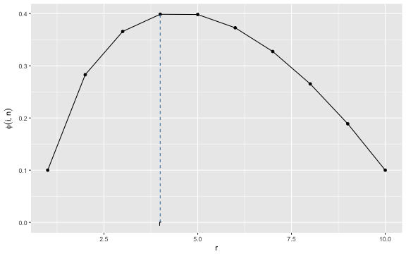
We can illustrate \(\phi_n(r)\) as a function of \(r\):

We thus select the \(r\), which
gives the highest value of \(\phi_n(r)\). In the example with \(n=10\) the best choice is \(r=
4\). We wrap these two steps into a function find_r(n),
which given n returns the best choice r. In
the example we therefore look at \(r-1=\)find_r(10)-1\(=3\) candidates in order to get a
baseline and then take the first candidate, which is better
than this baseline. In code this corresponds to:
(pickIdx <- which.max(relrank(x)[r:n] == 1 | (r:n == n)))## [1] 3x[pickIdx + (r-1)]## [1] 1In the example we thus actually manage to select the best candidate! However, this is not always guaranteed: for example, if the best overall candidate is among the training sample (4/10 chance for this to happen) we would end up with the last candidate flat no matter how good or bad it is. As stated above: the probability that the above decision strategy will pick the best candidate is \(\phi_{10}(4)=0.40\).
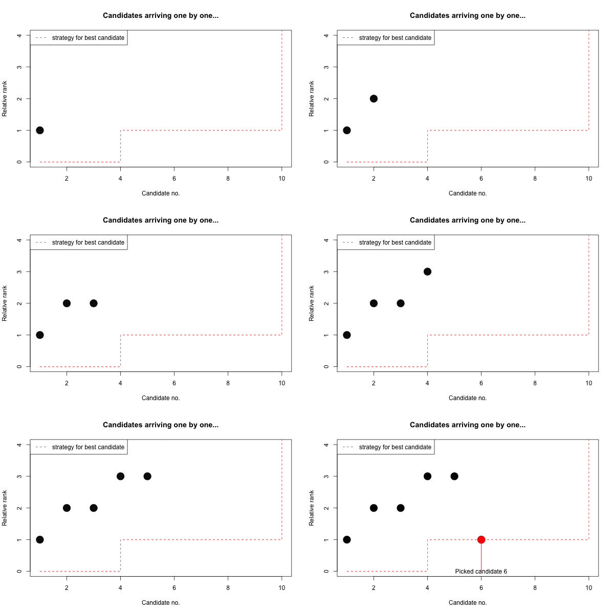
In order to compare the decision strategy with later formulations we denote by \(\mathbf{s}=(s_1,\ldots,s_n)\) a strategy which at time \(i\) selects candidate \(i\), if \(y_i \leq s_i\). In other words, the above strategy for \(n=10\) is:
s <- c(rep(0,r-1),rep(1,n-(r-1)-1),n)
s
## [1] 0 0 0 1 1 1 1 1 1 10And the selected candidate can easily found as
which.max(y <= s)## [1] 6For small \(n\) the optimal \(r\) and corresponding probability of success can easily be computed numerically. However, for large \(n\) the numerical precision as well as the computations become more tedious and hence interest is in finding a general asymptotic approximation as \(n\) grows large: One can show that as \(n\) gets large the optimal procedure is always to screen the first \(1/e\) = 37% and then select the first candidate better than the training sample (Gilbert and Mosteller 1966). The asymptotic probability of success, i.e. finding the overall best candidate, when following the such a procedure is also about \(1/e\)=37% (Gilbert and Mosteller 1966). Below we show a small table illustrating the precision of the asymptotic approximation.
| \(n\) | \(r-1\) | \((r-1)/n\) (%) |
|---|---|---|
| 10 | 4 | 40.0 |
| 100 | 38 | 38.0 |
| 1000 | 369 | 36.9 |
| 10000 | 3680 | 36.8 |
We summarise our above findings for how to find the best candidate in the following function:
strategy_best <- function(n) {
  r <- find_r(n)
  s <- c(rep(0,r-1),rep(1,n-(r-1)-1),n)
  return(s)
}

(s <- strategy_best(n))
## [1] 0 0 0 1 1 1 1 1 1 10…and sometimes one animation says more than a lot of text and equations:

Maximizing the expected rank
As attractive as it may sound, finding the overall best candidate appears a pedant’s criterion. In reality, you would typically settle with a lesser rank, as long as you know the candidate is good and it’s yours to keep. Hence, finding a satisficing strategy to minimize, e.g., the expected rank appears a more prudent objective for the risk adverse decision maker. This problem was addressed by Chow et al. (1964), we shall follow their treatment in what follows.
In their paper they show that the relative ranks \(y_1,\ldots,y_n\) are independent and the probability mass function of the \(i\)’s relative rank is \(P(y_i=j)=1/i\), \(j=1,\ldots,i\). Furthermore, the sequence of relative ranks has the Markov property and, hence,
\[ P(x_i=k|y_1=j_1,\ldots,y_{i-1}=j_{i-1},y_i=j) = P(x_i=k|y_i=j) = \frac{\binom{k-1}{j-1} \binom{n-k}{i-j}}{\binom{n}{i}}. \]
From this one computes
\[ E(x_i|y_i=j) = \sum_{k=1}^n k\cdot P(x_i=k|y_i=j) = \frac{n+1}{i+1} j. \]
Define \(c_i=c_i(n)\) to be the minimal possible expected overall rank selected if we limit us to strategies of the following type: use the first \(i\) candidates to generate a baseline and then, starting from \(i+1\), select the first candidate better than the baseline. Chow et al. (1964) shows that \(c_i\) can be computed by backwards recursion: Beginning with
\[
c_{n-1} = E\left(\frac{n+1}{n+1}y_n\right) = \frac{1}{n} \sum_{j=1}^n
j = \frac{n+1}{2},
\] and then for \(i=n-1,n-2,\ldots,1\) letting \[
s_i = \left[ \frac{i+1}{n+1} c_i\right] \\
c_{i-1} = \frac{1}{i} \left[ \frac{n+1}{i+1} \cdot \frac{s_i(s_i+1)}{2}+
(i-s_i)c_i \right],
\] where \([x]\) denotes the
largest integer smaller or equal to \(x\), i.e. floor(x). Because at
each decision time \(i\) we choose
between either picking the current candidate or proceeding to the next
candidate, we can evaluate the two options according to their expected
payoff:
- if we decide to wait deciding for at least another round the expected payoff is \(c_i\)
- If we selected the current candidate, which has relative rank \(y_i=j\) our expected payoff is \(E(x_i|y_i=j)\)
Our optimal stopping time is thus
\[ \min_{i\in \{1,\ldots,n\}} \{ E(x_i|y_i=j) \geq c_{i} \> \text{or} \> i=n \}. \]
Implicitly, the above computed sequence of \(s_i\)’s actually contains the resulting decision strategy (Chow et al. 1964). We transfer the procedure into R code as follows:
# Function to find a strategy minimizing expected rank as done by Chow et al. (1964).
strategy_erank <- function(n) {
  c <- s <- rep(NA,n)
  idx <- function(i) {i+1}
  c[idx(n-1)] <- (n+1)/2
  s[idx(n)] <- n

  for (i in (n-1):1) {
    s[idx(i)]   <- floor( (i+1)/(n+1)*c[idx(i)])
    c[idx(i)-1] <- 1/i * ( (n+1)/(i+1)*s[idx(i)]*(s[idx(i)]+1)/2 + (i-s[idx(i)])*c[idx(i)])
  }

  return(list(s=s,c=c))
}

print(strategy_erank(n),digits=4)
## $s
## [1] NA 0 0 0 1 1 2 2 3 5 10
##
## $c
## [1] 2.558 2.558 2.558 2.558 2.677 2.888 3.154 3.590 4.278 5.500Note that in the above, the first element of the vectors
s and c is the element 0. Hence, \(s_1\) is located at position two of the
vector. It is interesting to observe that for the example one forms a
baseline for the same amount of time, but after a while becomes more
desperate and accepts candidates who are not
optimal.
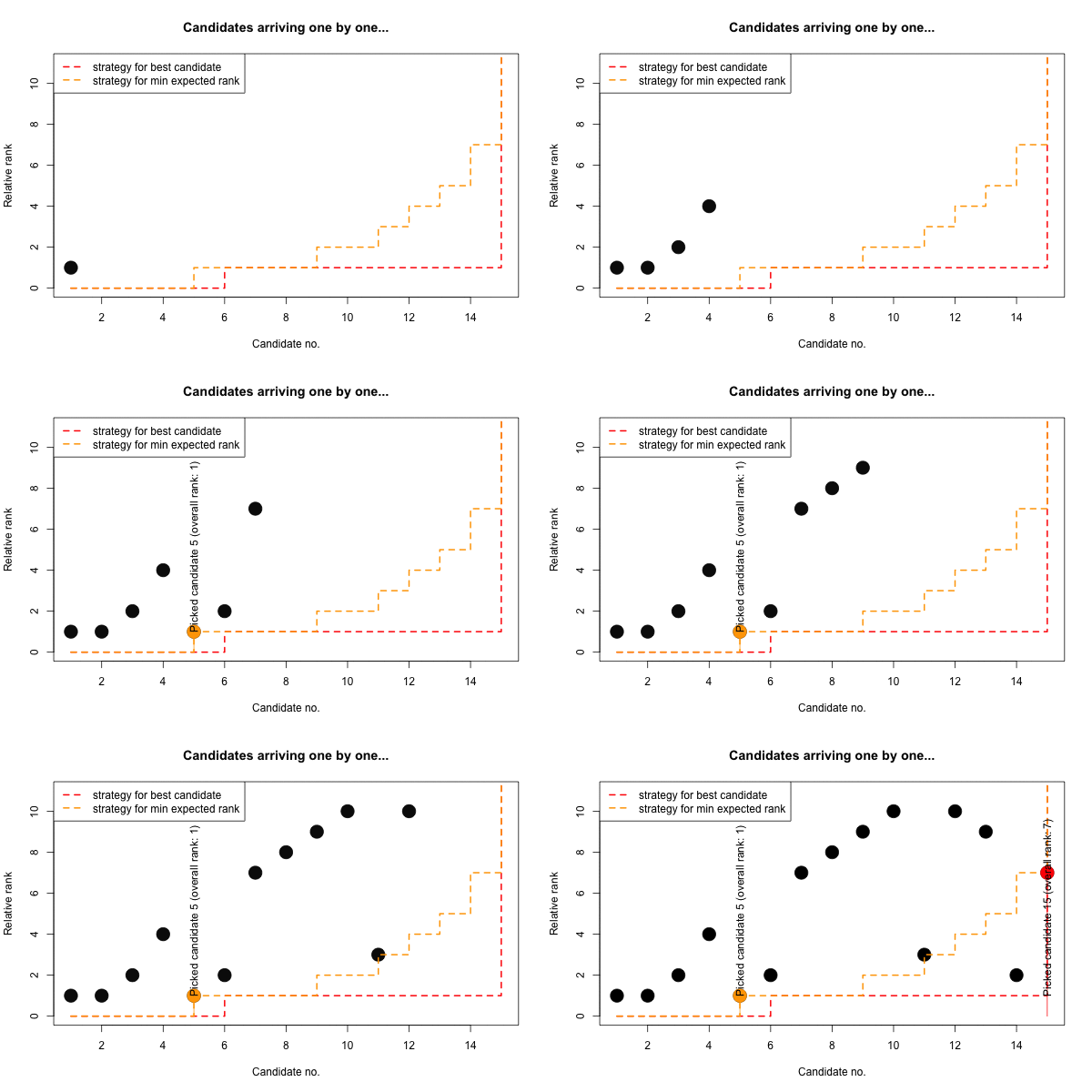
Finally, it is interesting to compare the two strategies for any \(n\) we like, e.g. \(n=15\):
(two_s <- rbind(best=strategy_best(n=15), erank=strategy_erank(n=15)$s[-1]))## [,1] [,2] [,3] [,4] [,5] [,6] [,7] [,8] [,9] [,10] [,11] [,12] [,13] [,14] [,15]
## best 0 0 0 0 0 1 1 1 1 1 1 1 1 1 15
## erank 0 0 0 0 1 1 1 1 2 2 3 4 5 7 15Again, for the expected minimizing rank strategy our training sample is slightly smaller than for the selecting the best strategy. Furthermore, we again adapt our relative-rank criterion as one becomes more desperate towards the end. Finally, we illustrate the two strategies on the \(n=15\) sequence with ranks \(x\) (and resulting relative ranks \(y\)):
##   [,1] [,2] [,3] [,4] [,5] [,6] [,7] [,8] [,9] [,10] [,11] [,12] [,13] [,14] [,15]
## x    8    5    6    9    1    3   10   12   14    15     4    13    11     2     7
## y    1    1    2    4    1    2    7    8    9    10     3    10     9     2     7
Monte Carlo simulation
Using Monte Carlo integration we can for a given \(n\) compute the expected rank obtained by each of the strategies.
simulate <- function(s,n) {
  x <- sample(seq_len(n),size=n,replace=FALSE)
  y <- relrank(x)
  idxSelect <- which.max(y <= s)
  return(c(rank=x[idxSelect],idx=idxSelect,isBest=(x[idxSelect]==1)))
}

strategies <- list(s_best=strategy_best(n), s_erank=strategy_erank(n)$s[-1])
res <- lapply(strategies, function(s) replicate(1e5, simulate(s=s,n=n)))
(sim <- rbind(best=apply(res[[1]], 1,mean), erank=apply(res[[2]],1,mean)))## rank idx isBest
## best 3.02481 6.98755 0.39855
## erank 2.55563 6.27949 0.33177From the results it becomes clear that the expected rank optimizing
strategy on average takes a little less time before selecting a
candidate. Furthermore, the obtained expected rank is somewhat better
than for the overall best decision strategy. We can also compare the
Monte Carlo estimate sim["erank","rank"]=2.556 against the
theoretical value of \(c_0\)=2.558.
Discussion
Is the blog title Mathematical advice for real life an
oxymoron? Certainly not! Assumptions 1-6 clearly state
the abstraction. You may not agree with these assumptions, but given
that framework, the two functions strategy_bestand
strategy_erank give practical advice for a certain class of
decisions. The methods are also clearly superior to Sheldon Cooper’s dice
strategy. Furthermore, assumptions 1-6 have been improved upon in a
multitude of ways (Freeman 1983). For example:
- unknown \(n\) or random \(n\sim\operatorname{Po}(\lambda)\)
- the opportunity to return to previous candidates, but with a probability \(p\) of being rejected
- Candidate score originating from a known underlying distribution, e.g. the uniform or the normal
- Candidate score originating from an \(U(a,b)\) uniform with unknown \(a<b\), but with a conjugate and sequentially updated bivariate Pareto prior on \((a,b)\)
Altogether, such methods provide decision support: One can evaluate a potential decision and compare results with other ways of reaching the decision. Frey and Eichenberger (1996) discuss that for marriage decisions investigations show that individuals decide rather quickly marrying the first reasonably serious partner. Where does this misalignment between theory and practice originate from? Some of it appears to be consequences of additional effects not addressed by the model, e.g., little marginal gain of searching longer, lemon effects, satisficing, endowment effects, etc… Life is complicated. Finding a satisficing complexity representation is non-trivial - even for mathematicians. :-)
