\[ \newcommand{\bm}[1]{\boldsymbol{\mathbf{#1}}} \DeclareMathOperator*{\argmin}{arg\,min} \DeclareMathOperator*{\argmax}{arg\,max} \]

Abstract

We discuss the computation of confidence intervals for the median or any other quantile in R. In particular we are interested in the interpolated order statistic approach suggested by Hettmansperger and Sheather (1986) and Nyblom (1992). In order to make the methods available to a greater audience we provide an implementation of these methods in the R package quantileCI and a small simulation study is conducted to show that these intervals indeed have a very good coverage. The study also shows that these intervals perform better than the currently available approaches in R. We therefore propose that these intervals should be used more in the future!

This work is licensed under a Creative Commons Attribution-ShareAlike 4.0 International License. The markdown+Rknitr source code of this blog is available under a GNU General Public License (GPL v3) license from github.

Introduction

Statistics 101 teaches that for a distribution, possibly contaminated with outliers, a robust measure of the central tendency is the median. Not knowing this fact can make your analysis worthy to report in the newspaper (Google translate).

Higher quantiles of a distribution also have a long history as threshold for when to declare an observation an outlier. For example, growth curves for children illustrate how the quantiles of, e.g., the BMI distribution develop by age. Obesity is then for children defined as exceedance of the 97.7% quantile of the distribution at a particular age. Quantile regression is a non-parametric method to compute such curves and the statistical community has been quite busy lately investigating new ways to compute such quantile regressions models.

The focus of this blog post is nevertheless the simplest setting: Given an iid. sample \(\bm{x}\) of size \(n\) from a univariate and absolutely continuous distribution \(F\), how does one compute an estimate for the \(p\)-Quantile of \(F\) together with a corresponding two-sided \((1-\alpha)\cdot 100\%\) confidence interval for it?

The Point Estimate

Computing the quantile in a sample with statistical software is discussed in the excellent survey of Hyndman and Fan (1996). The simplest estimator is based on the order statistic of the sample, i.e. \(x_{(1)} < x_{(2)} < \cdots < x_{(n)}\). \[ \hat{x}_p = \min_{k} \left\{\hat{F}(x_{(k)}) \geq p\right\} = x_{(\lceil n \cdot p\rceil)}, \] where \(\hat{F}\) is the empirical cumulative distribution function of the sample. Since \(\hat{F}\) has jumps of size \(1/n\) the actual value of \(\hat{F}(\hat{x}_{p})\) can end up being somewhat larger than the desired \(p\). Therefore, Hyndman and Fan (1996) prefer estimators interpolating between the two values of the order statistic with \(\hat{F}\) just below and just above \(p\). It is interesting that even 20 years after, there still is no universally accepted way to do this in different statistical software and the type argument of the quantile function in R has been a close friend when comparing results with SPSS or Stata users. In what follows we will, however, stick with the simple \(x_{(\lceil n \cdot p\rceil)}\) estimator stated above.

Below is illustrated how one would use R to compute the, say, the 80% quantile of a sample using the above estimator. We can compute this either manually or using the quantile function with type=1:

##Make a tiny artificial dataset, say, the BMI z-score of 25 children
sort(x <- rnorm(25))

##  [1] -1.44090165 -1.40318433 -1.21953433 -0.95029549 -0.90398754 -0.66095890 -0.47801787
##  [8] -0.43976149 -0.36174823 -0.34116984 -0.33047704 -0.31576897 -0.28904542 -0.03789851
## [15] -0.03764990 -0.03377687  0.22121130  0.30331291  0.43716773  0.47435054  0.60897987
## [22]  0.64611097  1.20086374  1.52483138  2.67862782

##Define the quantile we want to consider
p <- 0.8
##Since we know the true distribution we can easily find the true quantile
(x_p <- qnorm(p))

## [1] 0.8416212

##Compute the estimates using the quantile function and manually
c(quantile=quantile(x, type=1, prob=p), manual=sort(x)[ceiling(length(x)*p)])

## quantile.80%       manual 
##    0.4743505    0.4743505

Confidence interval for the quantile

Besides the point estimate \(\hat{x}_p\) we also would like to report a two-sided \((1-\alpha)\cdot 100\%\) confidence interval \((x_p^{\text{l}}, x_p^{\text{u}})\) for the desired population quantile. The interval \((x_p^{\text{l}}, x_p^{\text{u}})\) should, hence, fulfill the following condition: \[ P( (x_p^{\text{l}}, x_p^{\text{u}}) \ni x_p) = 1 - \alpha, \] where we have used the “backwards” \(\in\) to stress the fact that it’s the interval which is random. Restricting the limits of this confidence intervals to be one of the realisations from the order statistics implies that we need to find indices \(d\) and \(e\) with \(d<e\) s.t. \[ P( x_{(d)} \leq x_p \leq x_{(e)}) \geq 1 - \alpha. \] Note that it may not be possible to achieve the desired coverage exactly in this case. For now we prefer the conservative choice of having to attain at least the desired coverage. Note that for \(1\leq r \leq n\) we have \[ \begin{align*} P( x_{(r)} \leq x_p) &= P(\text{at least $r$ observations are smaller than or equal to $x_p$}) \\ &= \sum_{k=r}^{n} P(\text{exactly $k$ observations are smaller than or equal to $x_p$}) \\ &= \sum_{k=r}^{n} {n \choose k} P(X \leq x_p)^k (1-P(X \leq x_p))^{n-k} \\ &= \sum_{k=r}^{n} {n \choose k} p^k (1-p)^{n-k} \\ &= 1 - \sum_{k=0}^{r-1} {n \choose k} p^k (1-p)^{n-k} \end{align*} \] In principle, we could now try out all possible \((d,e)\) combinations and for each interval investigate, whether it has the desired \(\geq 1-\alpha\) property. If several combinations achieve this criterion we would, e.g., take the interval having minimal length. This is what the MKmisc::quantileCI function does. However, the number of pairs to investigate is of order \(O(n^2)\), which for large \(n\) quickly becomes lengthy to compute. Instead, we compute an equi-tailed confidence interval by finding two one-sided \(1-\alpha/2\) intervals, i.e. we find \(d\) and \(e\) s.t. \(P(x_{(d)} \leq x_p) = 1-\alpha/2\) and \(P(x_p \geq x_{(e)}) = 1-\alpha/2\). In other words,

\[ \begin{align*} d &= \argmax P(x_{(r)} \leq x_p) \geq 1 - \frac{\alpha}{2} \\ &= \texttt{qbinom(alpha/2, size=n, prob=p)} \\ e &= \argmin P(x_p \geq x_{(r)}) \geq 1 - \frac{\alpha}{2} \\ &= \texttt{qbinom(1-alpha/2, size=n, prob=p) + 1} \end{align*} \]

Note that the problem can arise, that the above solutions are zero or \(n+1\), respectively. In this case one has to decide how to proceed. For an illustration of the above in case of the median see the post by @freakonometrics. Also note that the qbinom function uses the Cornish-Fisher Expansion to come up with an initial guess for the quantile, which is then refined by a numerical search. In other words, the function is of order \(O(1)\) and will, hence, be fast even for large \(n\).

When it comes to confidence intervals for quantiles the set of alternative implementations in R is extensive. Searching for this on CRAN, we found the following functionality:

There might even be more, but for now we are satisfied comparing just the above mentioned procedures:

as.numeric(jmuOutlier::quantileCI(x=x, probs=p, conf.level=0.95)[1,c("lower","upper")])
as.numeric(EnvStats::eqnpar(x=x, p=p, ci=TRUE, ci.method="exact",approx.conf.level=0.95)$interval$limits)
as.numeric(EnvStats::eqnpar(x=x, p=p, ci=TRUE, ci.method="normal.approx",approx.conf.level=0.95)$interval$limits)
as.numeric(asht::quantileTest(x=x,p=p,conf.level=0.95)$conf.int)

## [1] -0.03377687  1.52483138
## [1] 0.2212113 2.6786278
## [1] -0.03377687  1.52483138
## [1] -0.03377687  2.67862782

An impressive number of similar, but yet, different results! To add to the confusion here is our take at this as developed in the quantileCI package available from github:

devtools::install_github("hoehleatsu/quantileCI")

The package provides three methods for computing confidence intervals for quantiles:

quantileCI::quantile_confint_nyblom(x=x, p=p, conf.level=0.95,interpolate=FALSE)
quantileCI::quantile_confint_nyblom(x=x, p=p, conf.level=0.95,interpolate=TRUE)
quantileCI::quantile_confint_boot(x, p=p, conf.level=0.95,R=999, type=1)

## [1] -0.03377687  2.67862782
## [1] 0.07894831 1.54608644
## [1] -0.03377687  1.20086374

The first procedure with interpolate=FALSE implements the previously explained exact approach, which is also implemented in some of the other packages. However, when the interpolate argument is set to TRUE (the default), an additional interpolation step between the two neighbouring order statistics is performed as suggested in the work of Nyblom (1992), which extends work for the median by Hettmansperger and Sheather (1986) to arbitrary quantiles. It generates intervals of the form:

\[ \left( (1-\lambda_1) x_{(d)} + \lambda_1 x_{(d+1)}, (1-\lambda_2) x_{(e-1)} + \lambda_1 x_{(e)} \right) \]

with \(0 \leq \lambda_1, \lambda_2 \leq 1\) chosen appropriately to get as close to the desired coverage as possible without knowing the exact underlying distribution - see the paper for details.

The last call in the above is to a basic bootstrap procedure, which resamples the data with replacement, computes the quantile using type=1 and then reports the 2.5% and 97.5% percentiles of this bootstrapped distribution. Such percentiles of the basic bootstrap are a popular way to get confidence intervals for the quantile, e.g., this is what we have used in Höhle and Höhle (2009) for reporting the 95% quantile of the absolute difference in height at so called check points in the assessment of accuracy for a digital elevation model (DEM) in photogrammetry. However, the coverage of the percentile bootstrap procedure is not without problems, because the convergence rate as a function of the number of replicates \(r\) is only of order \(O(r^{-\frac{1}{2}})\) for quantiles (Falk and Kaufmann (1991)). As a trade-off between accuracy and speed we use \(R=999\) throughout this post.

Simulation Study to Determine Coverage

We write a function, which for a given sample x computes two-sided confidence intervals for the p-Quantile using a selection of the above described procedures:

quantile_confints(x, p=p, conf.level=0.95)

##   jmuOutlier_exact EnvStats_exact EnvStats_asymp asht_quantTest nyblom_exact
## 1      -0.03377687      0.2212113    -0.03377687    -0.03377687  -0.03377687
## 2       1.52483138      2.6786278     1.52483138     2.67862782   2.67862782
##   nyblom_interp        boot
## 1    0.07894831 -0.03377687
## 2    1.54608644  1.49641655

In order to evaluate the various methods and implementations we conduct a Monte Carlo simulation study to assess each methods’ coverage. For this purpose we write a small wrapper function to conduct the simulation study using parallel computation. The function wraps the quantileCI::qci_coverage_one_sim function, which lets the user define a simulation scenario (true underlying distribution, size of the sample, etc.), then applies all confidence interval methods gathered in the above quantile_confints and finally assesses whether each confidence interval covers the true value or not.

simulate.coverage_qci <- function(n=n,p=p,conf.level=0.9, nSim=10e3, ...) {
  ##Windows users: change to below lapply function or use snow.
  ##lapplyFun <- function(x, mc.cores=NA, ...) pblapply(x, ...)
  lapplyFun <- parallel::mclapply

  sims <- dplyr::bind_rows(
    lapplyFun(1L:nSim, function(i) {
      quantileCI::qci_coverage_one_sim(qci_fun=quantile_confints, n=n,p=p,conf.level=conf.level,...)
    }, mc.cores = parallel::detectCores() - 1)
  ) %>% summarise(across(everything(), mean))
  return(sims)
}

Simulation 1

We can now compare the coverage of the different implementation for the particular n=25 and p=0.8 setting:

simulate.coverage_qci(n=25, p=0.8, conf.level=0.95)

##   jmuOutlier_exact EnvStats_exact EnvStats_asymp asht_quantTest nyblom_exact
## 1           0.9552         0.9461         0.9552         0.9786       0.9786
##   nyblom_interp   boot
## 1        0.9495 0.9198

Note that the nyblom_interp procedure is closer to the nominal coverage than it’s exact cousin nyblom_exact and the worst results are obtained by the bootstrap percentile method. We also note that the results of the jmuOutlier_exact method appear to deviate from asht_quantTest as well as nyblom_exact, which is surprising, because they should implement the same approach.

Simulation 2

As a further test-case we consider the situation for the median in a smaller sample:

simulate.coverage_qci(n=11, p=0.5, conf.level=0.95)

##   jmuOutlier_exact EnvStats_exact EnvStats_asymp asht_quantTest nyblom_exact
## 1           0.9873         0.9332         0.9583         0.9873       0.9873
##   nyblom_interp   boot hs_interp
## 1        0.9463 0.9332    0.9463

We note that the EnvStats_exact procedure again has a lower coverage than the nominal required level, it must therefore implement a slightly different procedure than expected. That coverage is less than the nominal for an exact method is, however, still somewhat surprising.

Edit 2019-05-14: I pointed the package maintainer to this problem after looking at the code. Versions larger than 2.1.1 of the EnvStats pkg now contain an updated version of this function and also the Nyblom function.

In this study for the median, the original Hettmansperger and Sheather (1986) procedure implemented in quantileCI as function median_confint_hs is also included in the comparison (hs_interp). Note that the Nyblom (1992) procedure for \(p=\frac{1}{2}\) just boils down to this approach. Since the neighbouring order statistics are combined using a weighted mean, the actual level is just close to the nominal level. It can, as observed for the above setting, be slightly lower than the nominal level. The bootstrap method again doesn’t look too impressive.

Simulation 3

We finally also add one of the scenarios from Table 1 of the Nyblom (1992) paper, which allows us to check our implementation against the numerical integration performed in the paper to assess coverage.

simulate.coverage_qci(n=11, p=0.25, conf.level=0.90)

##   jmuOutlier_exact EnvStats_exact EnvStats_asymp asht_quantTest nyblom_exact
## 1           0.9219         0.7633          0.841         0.9219       0.9219
##   nyblom_interp   boot
## 1        0.9014 0.8816

In particular the results of EnvStats_exact look disturbing. The coverage of the interpolated order statistic approach again looks convincing.

Simulation 4

Finally, a setup with a large sample, but now with the t-distribution with one degree of freedom:

simulate.coverage_qci(n=101, p=0.9, rfunc=rt, qfunc=qt, conf.level=0.95, df=1)

##   jmuOutlier_exact EnvStats_exact EnvStats_asymp asht_quantTest nyblom_exact
## 1           0.9547         0.9352         0.9547         0.9547       0.9547
##   nyblom_interp   boot
## 1        0.9495 0.9362

Again the interpolation method provides the most convincing results. The bootstrap on the other hand again has the worst coverage, a larger \(R\) might have helped here, but would have made the simulation study even more time consuming.

Conclusion and Future Work

Can we based on the above recommend one procedure to use in practice? Well, even though the simulation study is small, the exact EnvStats::eqnpar approach appears to yield below nominal coverage intervals, sometimes even substantially, and hence is not recommended in versions below or equal to 2.1.1 ¹. On the other hand, jmuOutlier_exact, asht_quantTest, and nyblom_exact in all four cases provide above nominal level coverage, i.e. the intervals are conservative in as much as they are too wide. Also slightly disturbing is that the results of the exact confidence interval methods varied somewhat between the different R implementations. Part of the differences arise from handling the discreteness of the procedure as well as the edge cases differently. The basic percentile bootstrap method is a simple approach, providing acceptable, but not optimal coverage and also depends in part on \(R\). In particular for very large \(n\) or for a large number of replication in the simulation study, the method with a large \(R\) can be slow. Suggestions exist in the literature on how to improve the speed of coverage convergence by smoothing (see, e.g., De Angelis, Hall, and Young (1993)), but such work is beyond the scope of this post.

The Hettmansperger and Sheather (1986) and Nyblom (1992) method, respectively, provide very good coverage close to the nominal level. The method is fast to compute, available through the quantileCI R package and would be our recommendation to use in practice.

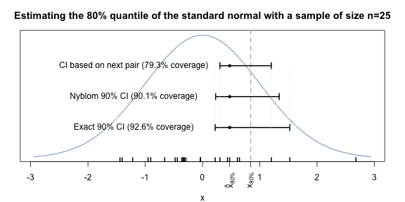
Altogether, we summarise our findings as follows: More confidence in confidence intervals for quantiles! and let the following picture illustrating 90% confidence intervals for the 80% quantile of the standard normal distribution based on the above sample of size \(n\)=25 say this in less than 1000 words.

Appendix

Given PDF \(f\) and CDF \(F\) of the underlying distribution, the coverage probability of the one sided Nyblom \((1-\alpha/2)\cdot 100\%\) confidence interval \((1-\lambda) x_{(r)} + \lambda x_{(r+1)}\) for \(x_p\) can be found as follows: Let \(z = (1-\lambda) x_{(r)} + \lambda x_{(r+1)}\). If the considered interval is a lower-confidence interval, we are interested in finding \(P( z \leq x_p)=\int_{-\infty}^{x_p} f_z(z) dz\). Here, the PDF of \(z\) is found as

\[ f_z(z) = \int_{-\infty}^{z} f_{x_{(r)},x_{(r+1)}}( x_{(r)}, x_{(r+1)}^*) dx_{(r)}, \quad\text{where}\quad x_{(r+1)}^* = \frac{z-(1-\lambda)x_{(r)}}{\lambda}. \]

The joint distribution of the order statistic is here

\[ f_{x_{(r)},x_{(r+1)}}( x_{(r)}, x_{(r+1)}) = \frac{n!}{(r-1)!(n-r-1)!} F(x_{(r)})^{r-1} \left( 1- F(x_{(r+1)})\right)^{n-r-1} f(x_{(r+1)}) f(x_{(r)}). \] The two nested integrals can be solved by numerical integration using, e.g., the integral function.

References