Beware the Argument: The Flint Water Crisis and Quantiles

Abstract

If your tap water suddenly becomes brown while authorities claim everything is okay, you start to worry. Langkjær-Bain (2017) tells the Flint Water Crisis story from a statistical viewpoint: essentially the interest is in whether the 90th percentile in a sample of lead concentration measurements is above a certain threshold or not. We illustrate how to perform the necessary calculations with R’s quantile function and show that the type-argument of the function matters.

This work is licensed under a Creative Commons Attribution-ShareAlike 4.0 International License. The markdown+Rknitr source code of this blog is available under a GNU General Public License (GPL v3) license from github.

Introduction

In a recent Significance article, Langkjær-Bain (2017) tells the story about the Flint water crisis. In 2014 the city of Flint, Michigan, USA, decided to change its water supply to Flint River. Due to insufficient treatment of the water with corrosion inhibitors the lead concentration in the drinking water increased, because lead in the aging pipes leached into the water supply. This created serious health problems - as explained in this short video summary. In this blog post we investigate further the computation of the 90th percentile of the tap water lead concentration samples described in Langkjær-Bain (2017). Quantile estimation in this context has already been discussed in a recent blog entry entitled Quantiles and the Flint water crisis by Rick Wicklin.

The monitoring of drinking water in the US is regulated by the Lead and Copper Rule of the United States Environmental Protection Agency. The entire text of the rule is available as electronic code of federal regulation (e-CFR) Title 40: Protection of Environment, Part 141 - National Primary Drinking Water Regulations. In particular the regulation defines a sampling plan for collecting tap water samples. The size of the sample depends on the number of people the water system serves. In case this number is bigger than 100,000 a sample of 100 sites is needed. If there are 10,001-100,000 people served, then a sample from 60 sites is needed. For systems serving fewer than 10,000 sizes of 40, 20, 10 and 5 are defined - see §141.86(c) of the rule for details. Of interest for this blog post is that action needs to be taken, if too many of the samples are above a given threshold of 15 part per billion (ppb):

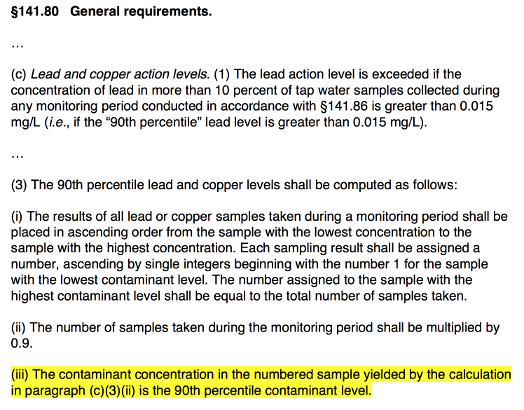
We note the explicit duality in the CFR between the in more than 10% and the 90% quantile in the text. However, we also note that it is not clear how to proceed, if the number calculated in (c)(3)(ii) is not an integer. This is not a problem per se, because the CFR itself only operates with samples sizes 100, 60, 40, 20, 10 and 5, where 0.9 times the sample size always gives an integer number. But if one for some reason does not obtain exactly the required number this quickly can become an issue as we shall see below.

The Flint Data

The data of the spring 2015 Flint water supply monitoring conducted by the Michigan Department of Environmental Quality are presented in the figure on p. 20 of Langkjær-Bain (2017). Alternatively, they can also be taken directly from the Blog entry Quantiles and the Flint water crisis by Rick Wicklin.

##Read flint water monitoring data (the column lead is the measurement)
flint <- read.csv(file=file.path(filePath,"flint.csv"))
##Sort the measured lead values in ascending order
lead  <- sort(flint$lead)
##Number of observations
n <- length(lead)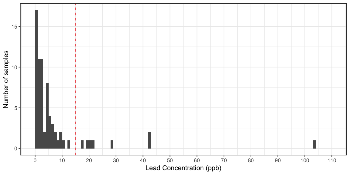

The proportion of observations above the 15 ppb threshold is

mean(lead > 15)

## [1] 0.1126761

In other words, the proportion 11.3% is above the 10% action threshold and, hence, something needs to be done. However, as Langkjær-Bain (2017) describes, the story is a little more complicated, because two of the values above 15 were removed with the argument that they originated from sites which are not covered by the sampling plan. Only private households at high risk, i.e. with lead pipelines, are supposed to be sampled. As one can read in the article the removal is highly controversial, in particular, because the proportion of critical observations falls below the 10% action threshold when these two values are removed. For this blog entry, we will, however, work with the full \(n=71\) sample and focus on the quantile aspect of the calculation.

Percentages and Quantiles

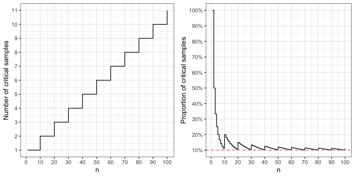
Let \(n\) denote the size of the selected sample, which in our case is \(n=71\). If more than 10% of the sample is to be above 15 ppb, this means that \(\lfloor 0.1\cdot n + 1\rfloor\) of the samples need to be above 15 ppb, where \(\lfloor y \rfloor\) denotes the largest integer less than or equal to \(y\). We shall denote this the number of critical samples. If we divide this number by \(n\) we get the actual proportion of critical samples needed before action. It is worthwhile noting the difference between this critical proportion and the 10% threshold illustrated by the sawtooth curve in the figure below. The explanation for these sawtooth step-spikes is the discreteness of the decision problem (i.e. \(x\) out of \(n\)).

Turning to the equivalent 90% quantile is above 15 ppm decision criterion of the CFR, one will need to determine the 90% quantile from the finite sample of lead concentration measurements. How to estimate quantiles with statistical software is discussed in the excellent survey of Hyndman and Fan (1996). In their work they describe the nine different quantile estimators implemented in R’s quantile function. The estimators are all based on the order statistic of the sample, i.e. let \(x_{(1)} \leq x_{(2)} < \cdots \leq x_{(n)}\) denote the ordered lead concentration measurements. Then the simplest estimator for the \(p\cdot 100\%\) quantile is

\[ \hat{x}_p = \min_{k} \left\{\hat{F}(x_{(k)}) \geq p\right\} = x_{(\lceil n \cdot p\rceil)}, \]

where \(\hat{F}\) is the empirical cumulative distribution function of the sample and \(\lceil y \rceil\) denotes the smallest integer greater than or equal to \(y\). This method corresponds to R’s type=1. For our application \(p\) would be 0.9 and the 90th percentile for the Flint data is thus

c("manual.90%"=lead[ceiling(n*p)], R=quantile(lead, probs=p, type=1))

## manual.90%      R.90% 
##         18         18

which is above the action threshold of 15 ppb. It is also important to note that when \(x_{(\lceil n \cdot 0.9\rceil)} > 15\> \text{ppb}\) then a total \(n - \lceil n \cdot 0.9\rceil + 1\) samples are above 15 ppm. In other words the proportion of samples above 15 ppm in this situation is \[ \frac{n - \lceil n \cdot 0.9\rceil + 1}{n}.\] To show the duality between the more than 10% critical samples and the 90% quantile being above 15 ppm we thus need to show that \((n - \lceil n \cdot 0.9\rceil + 1)/n = (\lfloor 0.1\cdot n + 1\rfloor)/n\). This is possible since the following relations hold for the floor and ceiling functions: \[ \begin{align*} - \lceil y \rceil &= \lfloor -y \rfloor \quad \text{and} \\ n + \lfloor y \rfloor &= \lfloor n + y \rfloor, \end{align*} \] with \(n\) being an integer and \(y\) any real number. Thus, \[ (n+1) - \lceil n \cdot 0.9\rceil = (n+1) + \lfloor -n \cdot 0.9\rfloor = \lfloor (n+1) - n \cdot 0.9\rfloor = \lfloor 0.1n+1 \rfloor. \]

Important conclusion: We have thus shown that with the type=1 quantile method we have the duality between having more than 10% critical samples and the 90th percentile of the measurements being above 15 ppm.

Other Quantile Types

Since \(\hat{F}\) has jumps of size \(1/n\) the actual value of \(\hat{F}(\hat{x}_{p})\) can end up being somewhat larger than the desired \(p\). Therefore, Hyndman and Fan (1996) prefer estimators interpolating between two adjacent order statistics. Also because such estimators have a lower mean squared error in most cases (Dielman, Lowry, and Pfaffenberger 1994). As an example of such an extended estimator, the type=5 quantile estimator is defined by letting \(h=p n + 1/2\) and then computing: \[ \hat{x}_p = x_{\lfloor h \rfloor} + (h - \lfloor h \rfloor) (x_{\lfloor h \rfloor + 1} - x_{\lfloor h \rfloor}). \]

Doing this either manually or using the quantile function one obtains:

## Small function to manually compute the type=5 p*100th quantile
## for the sample x
manual_quantile_5 <- function(x, p) {
  h <- length(x)*p + 0.5
  x <- sort(x)
  return(x[floor(h)] + (h - floor(h))* (x[floor(h)+1] - x[floor(h)]))
}

c("manual.90%"=manual_quantile_5(lead, p=0.9), R=quantile(lead, probs=0.9,type=5))

## manual.90%      R.90% 
##       18.8       18.8

Instead of reading the above or using the R code one can also instead watch a more didactic whiteboard explanation for Michigan Radio by Professor Christopher Gardiner on how to calculate the 90% quantile using a type=5 argument for the Flint sample. However, the important point of the above calculations is that this quantile type is of limited interest, because the Lead and Copper Rule implicitly defines that one has to use the type=1 quantile. To make this point even more explicit, we use sampling with replacement from the Flint data to construct a dataset, where the 90% type=5-quantile is above 15 ppm, but the percentage of samples above the 15 ppm threshold is less than 10%.

##Function to compute the proportion critical as well as the 90% quantile
##using type (type)-quantiles. Returns the quantile as well as the proportion
##above the 15 ppm threshold
prop_critical_and_q90 <- function(x, type=5) {
  q90 <- as.numeric(quantile(x, type=type,probs=p))
  prop <- mean(x>15)
  c(q90=q90,prop= prop)
}

##Make 100 datasets by sampling with replacement
r <- data.frame(seed=seq_len(100)) %>% rowwise %>% do({
  set.seed(.$seed)
  newdata <- sample(lead, replace=TRUE)
  as.data.frame(seed=.$seed, t(prop_critical_and_q90(newdata)))
})

##Check which datasets violate the duality between quantile and
##percentage above threshold assumption
r %<>% mutate(violates_duality =  q90 > 15 & prop < 0.1)

##Do the stats for this dataset
(five <- r %>% filter(violates_duality) %>% slice(1:5))

## Source: local data frame [5 x 3]
## Groups: <by row>
## 
## # A tibble: 5 x 3
##     q90   prop violates_duality
##   <dbl>  <dbl> <lgl>           
## 1  15.  0.0986 TRUE            
## 2  15.  0.0986 TRUE            
## 3  16.2 0.0986 TRUE            
## 4  15.  0.0986 TRUE            
## 5  15.8 0.0986 TRUE

We note that some of the lines in the above output are artifacts of lacking numerical precision: the quantile is only above 15 due to numerical imprecision in the calculation of the type=5 quantile:

print(five$q90, digits=20)

## [1] 15.000000000000028422 15.000000000000028422 16.200000000000045475
## [4] 15.000000000000028422 15.800000000000039790

This shows that regulatory business with floating point arithmetic is tricky. As a step towards fixing the problem, one could redefine the greater and less than operators, respectively, to only compare up to numerical precision:

##Function to do numerical safe greater than comparision
"%greater%" <- function(x,y) {
  equal_up_to_numerical_precision <- isTRUE(all.equal(x,y))
  return( (x > y) & !(equal_up_to_numerical_precision) )
}

##Function to do numerical safe less than  comparision
"%less%" <- function(x,y) {
  equal_up_to_numerical_precision <- isTRUE(all.equal(x,y))
  return( (x < y) & !(equal_up_to_numerical_precision) )
}

##Add the new column, which does < and > comparisons only up to
##numerical precision
r %<>% mutate(violates_duality_numsafe =  (q90 %greater% 15) & (prop %less% 0.1))

##Show five violation candidates for this corrected dataset
(five <- r %>% filter(violates_duality_numsafe) %>% slice(1:5))

## Source: local data frame [5 x 4]
## Groups: <by row>
## 
## # A tibble: 5 x 4
##     q90   prop violates_duality violates_duality_numsafe
##   <dbl>  <dbl> <lgl>            <lgl>                   
## 1  16.2 0.0986 TRUE             TRUE                    
## 2  15.8 0.0986 TRUE             TRUE                    
## 3  15.8 0.0986 TRUE             TRUE                    
## 4  16.2 0.0986 TRUE             TRUE                    
## 5  16.2 0.0986 TRUE             TRUE

Discussion

To summarize the findings: The type of quantile estimation used in practice matters. It is not clear what to do, if \(0.9\cdot n\) is not integer in the estimation of the 90% quantile under the Lead and Copper Rule. For the Flint example the 63’rd sorted value is 13 which is below threshold, whereas the 64’th value is 18 which is above the threshold. If we use type=1 then \(\lceil 71\cdot 0.9\rceil=64\) would be the correct value to take and the 90% quantile of the sample would be estimated to be 18 ppb. This means that the 19 ppb vertical line in the figure of Langkjær-Bain (2017) is a little misleading, because this appears to be the rounded type=5 quantile. For the setting with \(n=71\) samples, both estimators are although above the action threshold of 15 ppb, so in the particular Flint application it does not matter so much which method to take. However, in other settings this might very well make a difference! So be careful with the type argument of the quantile function. As an example, the nine different types of R’s quantile function provide estimates for the 90% quantile in the range from 17.50 to 19.60 for the Flint data. The default type argument in R is type=7, so if nothing else is specified when calling the quantile function type=7 is what you get.

On another note, one can discuss if it is a good idea to rely on the type=1 quantile estimator in the rule, because it is well known that this type does not have as good estimation properties as, e.g., type=5. However, type=1 is simpler to compute, ensures duality with the intuitive critical proportion, and has the property that the obtained value is always one also occurring in the sample. The later thus avoids the issue of numerical instability.

Finally, the blog post by Rick Wicklin addresses quantile estimation from an even more statistical viewpoint by computing confidence intervals for the quantile - a topic, which has been previously treated theoretically in this blog. Compliance to a given quantile threshold based on samples has also been treated in the entirely different context of digital elevation models (Höhle and Höhle 2009). Typically, tests and the dual confidence intervals are in this regulation setting formulated in a reversed way, such that one needs to provide enough evidence to show that underlying 90th percentile is indeed below 15 ppm beyond reasonable doubt. An interesting question in this context is how large the sample needs to be in order to do this with a given certainty - see Höhle and Höhle (2009) for details. It is, however, worthwhile pointing out that the Lead and Copper Rule does not know about confidence intervals. Currently, estimation uncertainty is only treated implicitly by specifying sample size as a function of number of people served by the water system and then hard-thresholding the result at 15 ppm.

Acknowledgments

Thanks goes to Brian Tarran, editor of the Significance Magazine, for providing additional information about the quantile computation of the Langkjær-Bain (2017) article and for pointing out the Gardiner video.

References