Confidence Intervals without Your Collaborator's Tears
Abstract
We provide an interpretation for the confidence interval for a binomial proportion hidden as the transcript of an hypothetical statistical consulting session.
 This work is licensed under a Creative Commons
Attribution-ShareAlike 4.0 International License. The
markdown+Rknitr source code of this blog is available under a GNU General Public
License (GPL v3) license from github.
This work is licensed under a Creative Commons
Attribution-ShareAlike 4.0 International License. The
markdown+Rknitr source code of this blog is available under a GNU General Public
License (GPL v3) license from github.
The Statistical Consulting Session
[Client]: So I did this important experiment where I investigated 420 turtles whether they had a specific phenotype trait. 52 out of my 420 turtles had the trait, i.e. the proportion in the sample was 12.4%. Now I’d like to state a 95% confidence interval for what the proportion of the trait is in the population of turtles (which is pretty large).
[Statistician]: Interesting, but no so fast. Before going into the statistical specifics I would like to talk about the representativeness of your sample. Can you explain in more detail what is the population of turtles you would like to make a statement about and how the sample was selected.
[Client]: I’m surprised you care about turtles (eyes start to glow). My research area is the indo-pacific subpopulation of the green sea turtle, in particular the one outside the Great Barrier Reef. The population is believed to be a few thousands large and we sample by catching turtles using the rodeo method at specific feeding grounds. Each turtle was then tagged and a skin biopsy was taken. From the biopsy it was determined if the turtle is clinically unhealthy by measuring marker values and then check if its specific value was outside the presented reference interval.
[Statistician]: Hmm, that’s a lot of information. And what population do you want to make a statement about? All green turtles?
[Client]: That would be nice, but no. There are genetic differences between the varies subspecies so I would be happy just to make a statement about the Great Barrier Reef population.
[Statistician]: That sounds fair. You might get some bias by only sampling from feeding grounds and I’m unsure about the spatial design of your capture strategy.
[Client:] We gave this a lot of thought and varied both the time and site of sampling, but there is no hypothesis that there is great spatial variation within the reef area.
[Statistician]: Well, it’s my job to check the
representativeness of the sample, but it sounds like you already gave
this great thought. From what you describe sampling appears to be
without replacement. However, since your population is large (and also
not really known), it appears acceptable to skip the finite population
correction. Since your sample is also pretty large, let’s therefore go
with the textbook large-sample confidence interval for a binomial
proportion, that is \(\hat{p} \pm 1.96
\sqrt{\hat{p}(1-\hat{p})/n}\), where \(\hat{p}=x/n\). Don’t worry about the
equation, let’s use R and the binom package to compute the
interval:
(ci <- binom::binom.asymp(x=x, n=n, conf.level=0.95))## method x n mean lower upper
## 1 asymptotic 52 420 0.1238095 0.09231031 0.1553087So the requested 95% CI is 9.2%- 15.5%. Happy?
[Client]: Well, yes, that looks nice, but I wonder how I can interpret the confidence interval. Is it correct to say that the interval denotes a region, which contains the true value with 95% probability?
[Statistician]: A confidence interval constructing procedure yields a random interval, because it depends on quantities (in particular \(x\)), which are random. However, once you plug-in the realization of the random variable (i.e. your observation), you get a realization of the confidence interval consisting of two numbers. Would we know the true value then we could tell, whether the value is covered by this particular interval or not. The specific interval we calculated above thus contains the true value with probability 0% or 100% - which of the two is the cases we unfortunately do not know.
The correct interpretation is thus that the confidence interval is constructed by a procedure, which, when you repeat the experiment many many times, is such that in 95% of the experiments the corresponding confidence interval would cover the true value. I can illustrate this using a small simulation study in R. Let’s assume your true proportion is 10%.
##Assumed true value of the proportion of turtles with the trait
theta_true <- 0.1

##Prepare data.frame with 10000 realizations of the experiment
df <- data.frame(x=rbinom(n=1e4, size=n, prob=theta_true))

##Compute 95% CI for each experiment
df %<>% do( {
  as.data.frame(cbind(.,rate=.$x/n,binom::binom.asymp(x=.$x, n=n)[c("lower","upper")]))
})
##Check if the interval covers the true value
df %<>% mutate(covers_true_value = lower < theta_true & upper > theta_true)

##Proportion of intervals covering the true value. This would be 95%
df %>% summarise(coverage = mean(covers_true_value))
## coverage
## 1 0.9446A graphic for the first 50 experiments shows their point estimates,
corresponding intervals and how they overlap the true value or not:
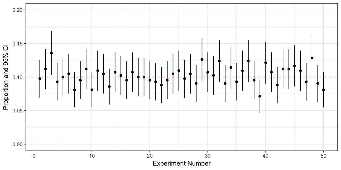
The specific confidence interval ci we computed above is
thus just one of many possible confidence intervals originating from the
above procedure.
[Client]: Ok, I get that is what happens when you do it many times. But I only have this one experiment with x = 52 out of n = 420 subjects having the trait of interest. Your above output does contain a very specific CI, with some very specific numbers, i.e. 9.2%- 15.5%. Is the true value in this interval with 95% probability?
[Statistician]: No, the realized interval either covers the true value or not. But since we do not know the true value it’s a bit like Schrödinger’s cat… To keep things very sketchy: The width of the interval gives you an indication of your estimation certainty, but the particular values are hard to interpret - except maybe as the critical limits in a corresponding hypothesis test. The later can loosely be interpreted as the range of parameters consistent with the data, where consistency is defined by a pre-defined type-I error probability.
[Client]: I’m sorry, but this is useless! You suggest to follow a common statistical protocol, you compute some numbers, but these numbers don’t really mean anything?
[Statistician]: Sorry, that’s the way it is. However, allow me to offer a different explanation: We both appear to agree that there is a true value of the proportion, right? Let’s denote this \(\theta\) with \(0 \leq \theta \leq 1\). We don’t know the true value, but we might have some prior idea about the range of plausible values for it. Would you be willing to characterize your belief about this by a distribution for \(\theta\)? This could be something as simple as assuming \(\theta \sim U(0,1)\), i.e. you would assume that every value of \(\theta\) between zero and one is equally probable initially. Then the interval we computed above denotes a 95% equal tail probability credibility region in a Bayesian framework when we assume this flat prior and use an asymptotic argument resulting in the posterior being Gaussian with the same mean and variance as the one would get from the asymptotic frequentist procedure.
[Client]: Umm, ok, but how’s that helpful?
[Statistician]: In the Bayesian context a 95% credibility region is a summary of your posterior belief about the parameter. Hence, it is ok to interpret this interval as that your belief after seeing the data is such that the true value is in that interval with 95% probability.
[Client]: I love this Bayes thing! This is what I wanted initially. But hang on, I don’t really believe in all values of the parameter being initially equally probable. I’ve seen some previous studies in the literature who under pretty similar conditions find that proportion is around 5-15%. How would I incorporate that?
[Statistician]: You could modify the large-sample Gaussian posterior such that it includes this prior information. Instead of using Gaussians you could alternatively also use a Beta distribution to perform so called conjugate prior-posterior updating of your belief about the true proportion. Let’s say the 5-15% denotes your prior 95% credibility region for the parameter. We would use this to find the parameters of a beta distribution. Then we would update your prior belief with the observed data to get the posterior distribution. A feature of such a conjugate approach is that this updated distribution, i.e. the posterior, is again beta. Doing this in R is easy:
##Function to determine beta parameters s.t. the 2.5% and 97.5% quantile match the specified values
target <- function(theta, prior_interval, alpha=0.05) {
  sum( (qbeta(c(alpha/2, 1-alpha/2), theta[1], theta[2]) - prior_interval)^2)
}

##Find the prior parameters
prior_params <- optim(c(10,10),target, prior_interval=c(0.05, 0.15))$par
prior_params
## [1] 12.04737 116.06022Actually, you can interpret the above prior parameters as the number of turtles you have seen with the trait (12) and without the trait (116), respectively, before conducting your above investigation. The posterior parameters are then 12 + 52 = 64 turtles with the trait and 116 + 368 = 484 turtles without the trait. You get the credible interval based on this posterior in R by:
##Compute credibile interval from a beta-binomial conjugate prior-posterior approach
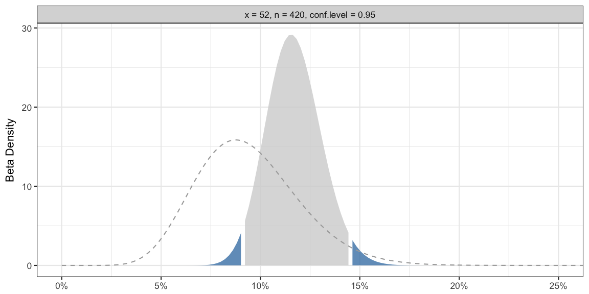
(ci_bayes <- binom::binom.bayes(x=x, n=n, type="central", prior.shape1=prior_params[1], prior.shape2=prior_params[2]))## method x n shape1 shape2 mean lower upper sig
## 1 bayes 52 420 64.04737 484.0602 0.1168518 0.09134069 0.1450096 0.05Graphically, your belief updating looks as follows:
##Plot of the beta-posterior
p <- binom::binom.bayes.densityplot(ci_bayes)
##Add plot of the beta-prior
df <- data.frame(x=seq(0,1,length=1000)) %>% mutate(pdf=dbeta(x, prior_params[1], prior_params[2]))
p + geom_line(data=df, aes(x=x, y=pdf), col="darkgray",lty=2) +
  coord_cartesian(xlim=c(0,0.25)) + scale_x_continuous(labels=scales::percent)
The dashed line in the graphic shows the density of your beta prior distribution. The shaded region shows the density of your beta posterior distribution, in particular, the gray shaded area denotes your 95% credibility region on the x-axis. One advantage of the beta-binomial approach is that this ensures that the prior as well as the posterior distribution have the same support as your parameter, i.e. the interval between zero and one.
[Client]: So I can really write that the interval 9.1%- 14.5% contains the true parameter with a probability of 95%?
[Statistician]: Depending on the technical level of your readership you might want to state that it’s a 95% equi-tailed credible interval resulting from a beta-binomial conjugate Bayesian approach obtained when using a prior beta with parameters such that the similar 95% equi-tailed prior credible interval has limits 0.05 and 0.15. Given these assumptions the interval 9.1%- 14.5% contains 95% of your subjective posterior density for the parameter.
[Client]: ???
[Statistician]: You might want to skip all the details and write that the 95% Bayesian confidence interval is 9.1%- 14.5%.
[Client]: And what if the reviewers do not agree with my prior distribution?
[Statistician]: Then return to your flat prior, i.e. the uniform. Nobody usually questions that even though you told me that you don’t believe in it yourself:
(ci_bayes_unif <- binom::binom.bayes(x=x, n=n, type="central", prior.shape1=1, prior.shape2=1))## method x n shape1 shape2 mean lower upper sig
## 1 bayes 52 420 53 369 0.1255924 0.09574062 0.158803 0.05[Client]: Alright, that’s settled then - I just use a Bayesian confidence interval with a flat prior and am done. That was not so hard after all. Now to something else, the reviewers of the paper, which by the way has to be revised by tomorrow, also asked us to substantiate our findings with a p-value. How would I get a p-value related to the above?
[Statistician]: Look how late it already is! I really need to go. I have this Bayesian Methods class to teach…