Judging Freehand Circle Drawing Competitions

Abstract:

In 2007 Alexander Overwijk went viral with his ‘Perfect Circle’ video. The same year a World Freehand Circle Drawing Championship was organized which he won. In this post we show how a mobile camera, R and the imager package can be used to develop an image analysis based method to judge future instances of the championship.

This work is licensed under a Creative Commons Attribution-ShareAlike 4.0 International License. The markdown+Rknitr source code of this blog is available under a GNU General Public License (GPL v3) license from github.

Introduction

A few years back I watched with awe the 2007 video of Alexander Overwijk’s freehand drawing a 1m diameter circle:

Ever since watching that video I have wondered how one would go about to judge the winner of such an alleged World Freehand Circle Drawing Championship (WFHCDC). While researching for this post I finally figured it out. On his web page Alexander in the story behind the video “reveals”:

They have a laser machine called the circleometer that creates the perfect circle closest to the one you drew. The circleometer then calculates the difference in area between the laser circle and the circle that you drew. The machine then calibrates the area difference as if you had drawn a circle with radius one meter. The person with the smallest area difference is declared the world freehand circle drawing champion.

Aha! Imaginary circleometers are expensive and my dean of study most likely isn’t open for investing in perfect circle measurement equipment… So here is a cheaper solution involving a mobile device camera, R and the imager package by Simon Barthelmé et al. Altogether a combination of modern data science tools, which my dean of study is most likely to approve! We’ll use a screenshot from the perfect circle video as motivating example to guide through the 3 phases of the method:

1. Image rectification
2. Freehand circle identification and perfect circle estimation
3. Quantifying deviation from the perfect circle

We start by loading the screenshot into R using imager:

library("imager")
file <- "circle2.png"
img <- imager::load.image(file.path(fullFigPath, file))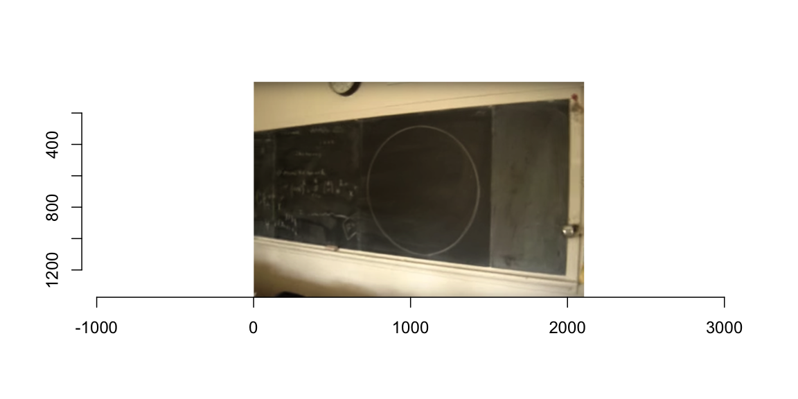

Image rectification

The image clearly suffers from perspective distortions caused by the camera being positioned to the right of the circle and, hence, not being orthogonal to the blackboard plane. Furthermore, small lense distortions are also visible - for example the right vertical line of the blackboard arcs slightly. Since the video contains no details about what sort of lense equipment was used, for the sake of simplicity, we will ignore lense distortions in this post. If such information is available one can use a program such as RawTherapee (available under a GNU GPL v3 license) to read the EXIF information in the meta data of the image and automatically correct for lens distortion.

To rectify the image we estimate the parameters of the 2D projection based on 4 ground control points (GPC). We use R’s locator function to determine the pixel location of the four corner points of the blackboard in the image, but could just as well use any image analysis program such as Gimp. Furthermore, we need the true object coordinates of these GPC. Unfortunately, these are only approximately available to due lack of knowledge of the size of the blackboard in the classroom. As a consequence a guesstimate of the horizontal length is used.

plot(img)
p <- locator(4)
p <- round(cbind(p$x, p$y))
dump(list=c("p"), "")

These points are now used to rectify the image by a Direct Linear Transformation (DLT) based on exactly 4 control points (Hartley and Zisserman 2004, chap. 4)¹. That is the parameters of the 3x3 transformation matrix \(H\) in homogeneous coordinates are estimated such that \(p' = H p\), see the code on github for details.

We can implement the rectifying transformation using the imager::warp function:

##Transform image coordinates (x',y') to (x,y), i.e. note we specify
##the back transformation p = H * p', so H here is the inverse.
map.persp.inv <- function(x,y, H) {
  out_image <- H %*% rbind(x,y,1)
  list(x=out_image[1,]/out_image[3,], y=out_image[2,]/out_image[3,])
}
##Pad dx_blackboard pixels to the right to make space for the blackboard coming closer
img_padded <- pad(img, nPix=dx_blackboard, axes="x", pos=1)
##Warp image
warp <- imwarp(img_padded, map=function(x,y) map.persp.inv(x,y,solve(H)),coordinates="absolute", direction="backward")

The result looks as follows: 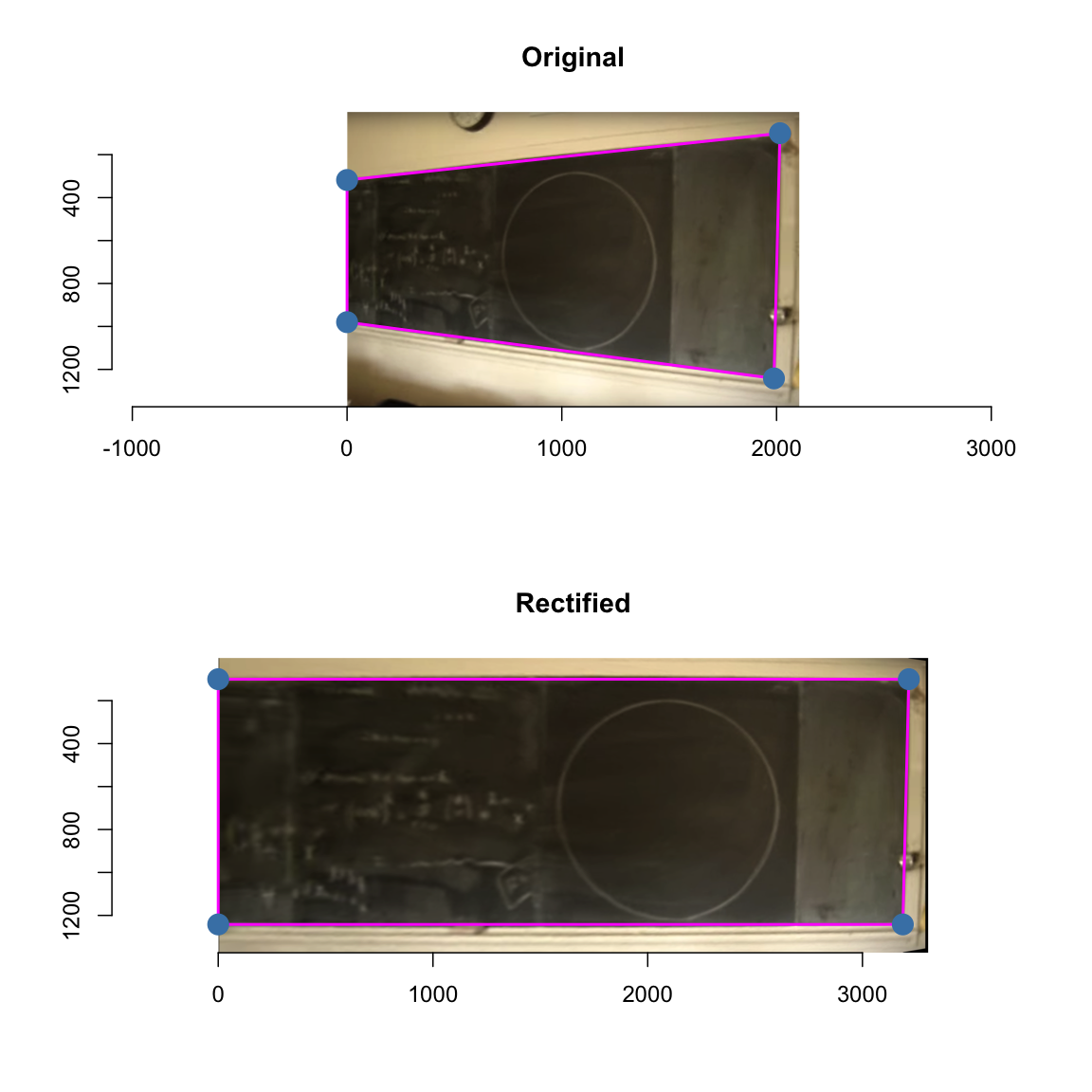Please notice the different x-axes of the two images when comparing them. For faster computation and better visualization in the remainder of this post, we crop the x-axis of the image to the relevant parts of the circle.

warp <- imsub(warp, x %inr% c(dx_blackboard, nrow(warp)))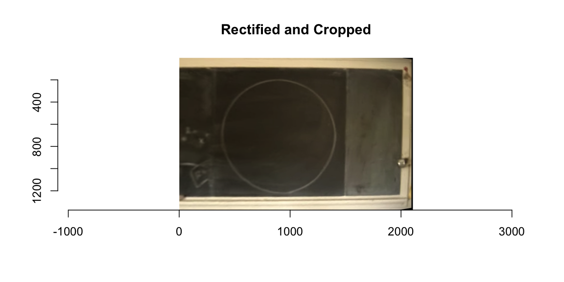

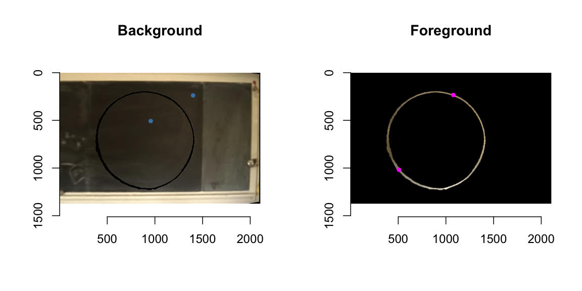
Freehand circle identification

As described in the imager edge detection tutorial we use length of the gradient to determine the edges in the image. This can be done by applying filters to the image.

##Edge detection function. Sigma is the size of the blur window.
detect.edges <- function(im, sigma=1) {
  isoblur(im,sigma) %>% imgradient("xy") %>% enorm() %>% imsplit("c") %>% add
}
#Edge detection filter sequence.
edges <- detect.edges(warp,1) %>% sqrt

To detect the circle from this we specify a few seed points for a watershed algorithm with a priority map inverse proportional to gradient magnitude. This includes a few points inside and outside the circle and a few points on the circle. Note: a perfect circle would have no border, but when drawing a circle with a piece of chalk it’s destined to have a thin border line.

We can now extract the circle by:

##Just the circle
freehandCircle <- (warp * (mask==2) > 0) %>% grayscale
##Total area covered by the circle
freehandDisc <- label(freehandCircle, high_connectivity=TRUE) > 0

…and by morphological operations we get just the outer border as a hairline

dilatedDisc <- freehandDisc %>% dilate_rect(sx=3,sy=3)
freehandCircleThinBorder <- (freehandDisc - dilatedDisc) != 0

Perfect circle estimation

Once the freehand circle path in the image has been identified, we need to find the best fitting perfect circle matching this path. This problem is elegantly solved by Coope (1993), who formulates the problem as finding center and radius of the circle minimizing the squared Euclidean distance to \(m\) data points \(a_j\), \(j=1,\ldots,m\). Denoting by \(c\) the center of the circle and by \(r>0\) the radius we want to find the solution of

\[ \min_{c\in \mathbb{R^2}, r>0} \sum_{j=1}^m F_j(c,r)^2, \quad\text{where}\quad F_j(c,r) = \left|r - ||c-a_j||_2\right|, \]

and \(||x||_2\) denotes Euclidean distance. Because the curve fitting minimizes the distance between an observed point \(a_j\) and its closest point on the circle and thus involves both the \(x\) and the \(y\) direction , this is a so called total least squares problem. The problem is non-linear and can only be solved by iterative numerical methods. However, the dimension of the parameter space can be reduced by one, because given the center \(c\) we can determine that \(r(c)=\frac{1}{m} \sum_{j=1}^m ||c-a_j||_2\).

##Compute radius given center
radius_given_center <- function(center, dist=NULL) {
  if (is.null(dist)) {
    a <- as.matrix(where(freehandCircleThinBorder > 0))
    dist <- sqrt((a[,1] - center[1])^2 + (a[,2] - center[2])^2)
  }
  return(mean(dist))
}

##Target functin of the total least squares criterion of Coope (1993)
target_tls <- function(theta) {
  ##Extract parameters
  center <- exp(theta[1:2])

  ##Total least squares criterion from Coope (1993)
  a <- as.matrix(where(freehandCircleThinBorder > 0))
  dist <- sqrt((a[,1] - center[1])^2 + (a[,2] - center[2])^2)
  ##Compute radius given center
  radius <- radius_given_center(center, dist)

  F <- abs( radius - dist)
  sum(F^2)
}


res_tls <- optim(par=log(c(x=background[1,1], y=background[1,2])), fn=target_tls)
center <- exp(res_tls$par)
fit_tls <- c(center,radius=radius_given_center(center))
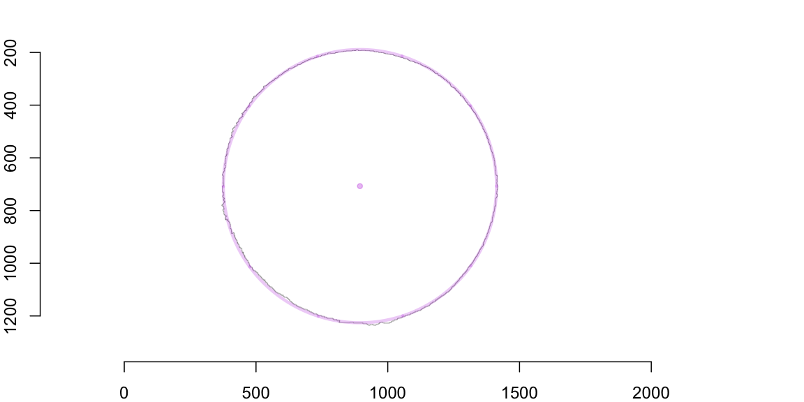
fit_tls

##        x        y   radius 
## 894.3885 707.3191 518.4119

We illustrate the freehand circle (in black) and the fitted circle (magenta) on top of each other using the alpha channel. You have to study the image carefully to detect differences between the two curves!

Quantifying the circularness of the freehand circle

We quantify the circularness of the freehand circle by contrasting the area covered by it with the area of the fitted perfect circle. The closer this ratio is to 1 the more perfect is the freehand circle.

##Area of the freehand drawn disc
areaFreehandDisc <- sum(freehandDisc)

##Area of the disc corresponding to the idealized circle fitted
##to the freehand circle
areaIdealDisc <- pi * fit_tls["radius"]^2

##Ratio between the two areas
ratio_area <- as.numeric(areaFreehandDisc  / areaIdealDisc)
ratio_area

## [1] 0.9971778

Yup, it’s a pretty perfect circle! Since the fitted circle already takes the desired shape into account, my intuition is that this ratio is a pretty good way to quantify circularness. However, to avoid measurehacks, we use as backup measure the circleometer approach: for each point on the freehand circle we measure its distance to the freehand circle and integrate/sum this up over the path of the freehand circle. We can approximate this integration using image pixels as follows.

##Create a pixel based circle in an image of the same size as the
##freehandCircle img. For visibility we use a border of 'border' pixels
##s.t. circle goes [radius - border/2, radius + border/2].
Circle <- function(center, radius, border) {
  as.cimg(function(x,y) {
    lhs <- (x-center[1])^2 + (y-center[2])^2
    return( (lhs >= (radius-border/2)^2) & (lhs <= (radius+border/2)^2))
  }, dim=dim(freehandCircle))
}

##Build pixel circle based on the fitted parameters
C_tls <- Circle(fit_tls[1:2], fit_tls[3], border=1)
##Calculate Euclidean distance to circle for each pixel in the image
dist <- distance_transform(C_tls, value=1, metric=2)
##Distance between outer border of freehand circle and perfect circle
area_difference <- sum(dist[freehandCircleThinBorder>0])

##Compute area difference and scaled it by the area of the fitted disc
ratio_areadifference <- as.numeric(area_difference / areaIdealDisc)

The image below illustrates this by overlaying the result on top of the distance map. For better visualization we zoom in on the 270-300 degree part of the circle (i.e. the bottom right). In magenta is the fitted perfect circle, in gray the freehand circle and the area between the two paths is summed up over the entire path of the freehand circle:

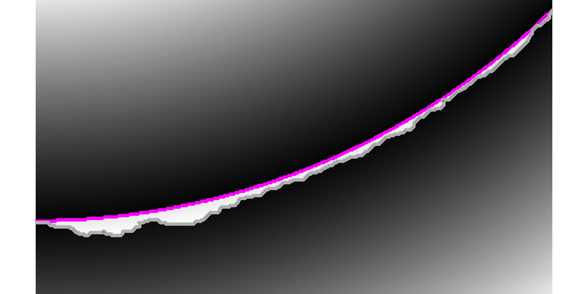
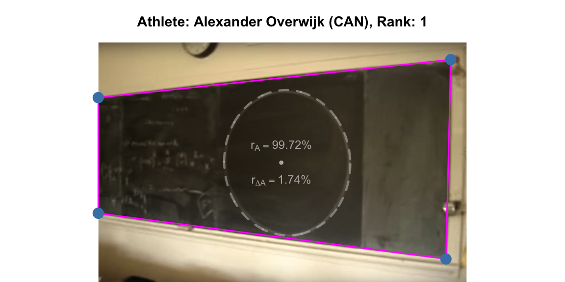
We obtain ratio_areadifference= 0.01735. Thus also this measure tells us: it’s a pretty perfect circle! To summarise: The output on the display of the judge’s Circle-O-Meter App (available under a GPL v3 license) at the World Freehand Circle Drawing Championship would be as follows: 😉

Discussion

We took elements of computer vision, image analysis and total least squares to segment a chalk-drawn circle on a blackboard and provided measures of it’s circularness. Since we did not have direct access to the measurements of the blackboard in object space, a little guesstimation was necessary, nevertheless, the results show that it was a pretty circular freehand circle!

With the machinery in place for judging freehand circles, its time to send out the call for contributions to the 2nd World Freehand Circle Drawing Championship (online edition). Stay tuned for the call: participants would upload their photo plus minor modifications of a general analysis R-script computing the two area ratios measures and submit their contribution by a pull request to the github WFHCDC repository. You can spend the anxious waiting time practicing your freehand 1m diameter circles - it’s a good way to loosen up long and unproductive meetings!

Appendix

If we instead of the total sum of squares criterion involving \(F_j(c,r)\) mentioned in the text solve the related criterion \[ \sum_{j=1}^m f_j(c,r)^2, \quad\text{where}\quad f_j(c,r) = ||c-a_j||_2^2 - r^2, \] then a much simpler solution emerges. Coope (1993) explains that this alternative criterion geometrically corresponds to minimizing the product

\[ \text{(distance to the closest point on the circle)}\times \text{(distance to the furthest away point point on the circle)} \]

over the measurement point. In order to obtain the solution write the residuals \(f_j\) as \(f_j(c,r) = c^T c - 2 c^T a_j + a_j^T a_j - r^2\) and perform a change of variables from \((c_1, c_2, r)'\) to \[ y = \left[ \begin{matrix} 2 c_1 \\ 2 c_2 \\ r^2 - c^T c \\ \end{matrix} \right] \quad \text{and let} \quad b_j = \left[ \begin{matrix} a_{j1} \\ a_{j2} \\ 1 \end{matrix} \right]. \] The minimization problem then becomes \[ \min_{y \in \mathbb{R}^3} \sum_{j=1}^m \left\{ a_j^T a_j - b_j^T y \right\}, \] which can be written as a linear least square (LLS) expression \[ \min_y ||By - d||_2^2, \] where \(B\) is a \(3\times m\) matrix with the \(b_j\)-vectors as columns and \(d=||a_j||_2^2\). This expression is then easily solved using the standard least squares machinery.

##Fast linear least squares problem as described in Coope (1993)
fitCircle_lls <- function(freehandCircle) {
  a <- as.matrix(where(freehandCircle > 0))
  b <- cbind(a,1)
  B <- b
  d <- a[,1]^2 + a[,2]^2
  y <- solve(t(B) %*% B) %*% t(B) %*% d
  x <- 1/2*y[1:2]
  r <- as.numeric(sqrt(y[3] + t(x) %*% x))
  return(c(x=x[1], y=x[2], radius=r))
}

##Fit using linear least squares procedure of Coole (1993)
fit_lls <- fitCircle_lls(freehandCircleThinBorder)

##Compare TLS and LLS fit
rbind(lls=fit_lls,tls=fit_tls)

##            x        y   radius
## lls 894.3666 707.3901 518.4295
## tls 894.3885 707.3191 518.4119

In other words: the results are nearly identical.

Literature