Is the answer to everything Gaussian?
Abstract:
As an applied statistician you get in touch with many challenging problems in need of a statistical solution. Often, your client/colleague already has a working solution and just wants to clarify a small statistical detail with you. Equally often, your intuition suggests you that the working solution is not statistically adequate, but how to substantiate this? As motivating example we use the statistical process control methodology used in Sarma et al. (2018) for monitoring a binomial proportion as part of a syndromic surveillance kit.

 This work is licensed under a Creative Commons
Attribution-ShareAlike 4.0 International License. The
markdown+Rknitr source code of this blog is available under a GNU General Public
License (GPL v3) license from github.
This work is licensed under a Creative Commons
Attribution-ShareAlike 4.0 International License. The
markdown+Rknitr source code of this blog is available under a GNU General Public
License (GPL v3) license from github.
Introduction
A few weeks ago I became aware of the publication by Sarma et al. (2018) who, as part of a syndromic surveillance system, monitor the time series of a proportion with the aim of timely detecting changes. What initially caught my intention was their figure 1A:
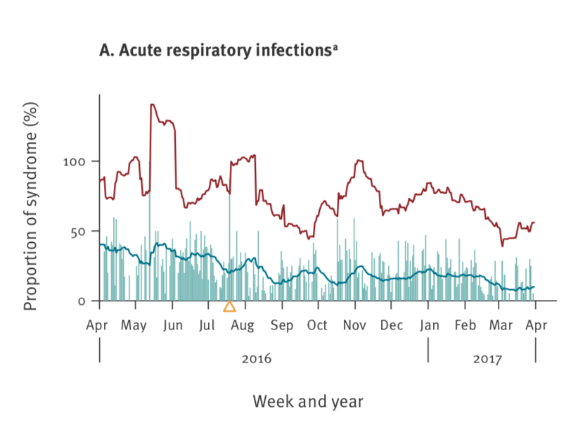
Reading the details of the paper reveals that the number of daily counts on 14 syndromes is collected and for each syndrome the proportion of the particular syndrome out of all syndrome reports is calculated. In other words: given that the counts for a particular day \(t\) are \(y_{it}, i=1, \ldots, 14\), the monitored proportion is \(p_{it} = y_{it}/\sum_{j=1}^{14} y_{jt}\). It is thus clear that it’s impossible to get beyond 100%. The more surprising was that the upper level in the figure goes beyond it - a sign of an inadequate statistical method. What the authors do is to compute an upper threshold for a particular day \(t_{0}\) as follows:
\[ U_{t_0} = \overline{p}_{t_0}(d) + k \cdot s_{t_0}(d), \quad \text{where}\\ \quad \overline{p}_{t_0}(d) = \frac{1}{d}\sum_{t=t_0-d}^{t_0-1} p_{t} \quad\text{and}\quad s_{t_0}(d) = \frac{1}{d-1} \sum_{t=t_0-d}^{t_0-1} (p_{t} - \overline{p}_{t_0}(d))^2 \]
is the mean and standard deviation of the \(d\) baseline observations1, respectively, and \(k\) is a tuning parameter - for 12 out of the 14 syndromes \(k=2\) is used, but for the two syndromes with highest proportions, including acute respiratory infections, \(k=4\) is used. As the method looks like an adaptation of the simple EARS method (Fricker, Hegler, and Dunfee 2008) to proportions, this caused me to tweet the following critical remark (no harm intended besides the scientific criticism of using a somewhat inadequate statistical method):
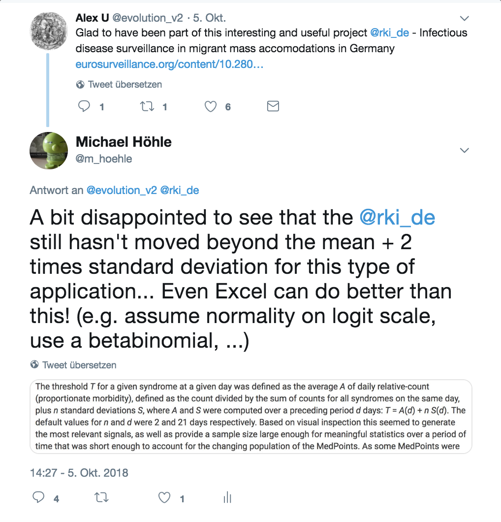
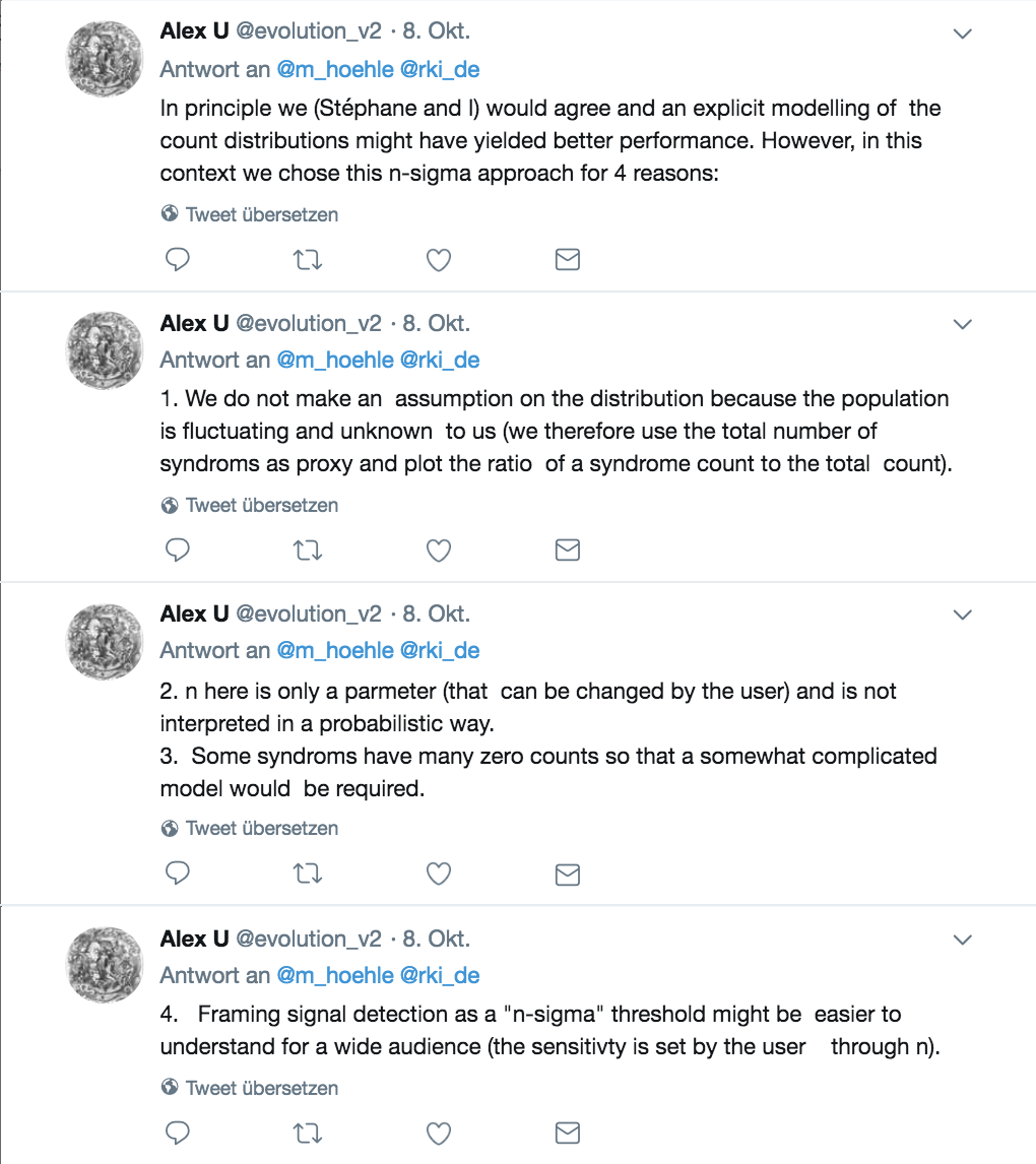
To which one of the authors, Alexander Ullrich, replied
Initially, I replied by twitter, but realized that twitter is not a good format for a well-balanced and thorough scientific discourse. Also, my answers lacked exemplification and supporting numbers, so I deleted the answers and shall instead use this blog post to provide a thorough answer. Please note that my discussion focuses on the paper’s statistical methodology approach - I do think the published application is very important and I’m happy to see that the resulting Excel tool is made available to a greater audience under a creative common license!
As much I can understand the motives, working in applied statistics is always a balance between mathematical exactness and pragmatism. A famous quote says that things should be as simple as possible, but not simpler. But if mathematical rigour always comes in second place, something is amiss. In this light, I’d like to comment on the four reasons given in Alexander’s reply.
Reason 1 & 2:
In principle I agree and taking a non-parametric and distribution free approach is healthy, if you fear your assumptions are more quickly violated than you can formulate them. Using the mean plus two times standard deviation of the \(d=15\) baseline proportions does, however, imply certain assumptions. It means that you believe i the distribution being sufficiently stable that the expectation and standard deviation estimated from the baseline values is indicative for the next observation’s expectation and standard deviation. In other words: no trends, no day of the week effects and no previous outbreaks are allowed in the baseline. Looking at the jump of the upper-bound line after the single peak in June 2016 in Fig 1A one concludes that this might be a problematic assumption. Furthermore, one assumes that the distribution is sufficiently symmetric such that its quantiles can be described as a number of times the standard deviations away from the mean. Finally, by using the usual formula to estimate the standard deviation one assumes that the observations are independent. They are likely not and, hence, the estimated standard deviation might be too small. All these limitations need to be mentioned and are probably the biggest problem with the method, but could be addressed by semi-simple modelling approaches as done, e.g., in (farrington96?) for counts.
For the remainder of this post, I shall instead focus on using the mean plus two times standard deviation (sd) rule, as I have seen it too many times - also in other surveilance contexts. The problem we are solving is a statistical one, so writing that the k-times-sd-rule is not meant to have a probabilistic interpretation leaves the user alone with the choice of threshold. In particular many users will know from their Statistics 101 class that mean plus/minus two times sd is as a way to get approximately 95% of the mass for anything which has a Gaussian shape. Due to the central limit theorem this shape will apply to a certain degree.
So what we do is to compare an out-of-sample observation with a threshold. In this case the prediction interval for the observation is the statistical correct object for the comparison. Because the standard deviation is estimated from data, the prediction interval should be based on quantiles of a t-distribution with \(d-1\) degrees of freedom. In this case the appropriate upper limit of a two-sided \((1-\alpha)\cdot 100%\) prediction interval is given as
\[ \begin{align} \label{eq:predict-ul-gauss} \ U_{t_0} = \overline{p}_{t_0}(d) + t_{1-\alpha/2}(d-1) \cdot \sqrt{1+\frac{1}{d}} \cdot s_{t_0}(d), \end{align} \] where \(t_{1-\alpha/2}(d-1)\) denotes the \(1-\alpha/2\) quantile of the t-distribution with \(d-1\) degrees of freedom. In our case \(\alpha=0.05\) so we need the 97.5% quantile. See for example Chapter 10 of Young and Smith (2005) or the Wikipedia page on prediction intervals for details.
With \(d=15\) 2 the upper limit of a one-sided 97.5% prediction interval would have the multiplication factor 2.22 on the estimated standard deviation. Using a factor of 2 instead means your procedure is slightly more sensitive than the possibly anticipated 2.5% false alarm probability. Calculations show that the false alarm probability under the null hypothesis is 3.7% (assuming the Gaussian assumption holds). For the sake of simplicity one can say that this difference in the \(d=15\) case appears ignorable. Had \(d\) been smaller the difference becomes more relevant though.
Reason 3
I’m not sure I got the point, but one problem is that if your baseline consists of the observations \(y\), \(y\), \(\ldots\), \(y\) then the upper limit by your method will also be \(y\), because the estimated standard deviation will be zero. Another problem is if the denominator \(n_t\) is zero, but because this appears to have a regular shape (no reports on weekends), this can just be left out of the modelling?
Reason 4
This reason I find particular troublesome, because it is an argument statisticians hear often. A wider audience expects a valid statistical method, not more complicated than necessary, but sound and available within the tools at hand. I argued above that two times standard deviation for proportions might be working, but you implicitly leave a lot of problems for the user to solve due to insufficient statistical modelling. I agree that too complicated might not work, but if -for the sake of pragmatism- we neither inform or quantify potential problems of a too simplistic solution nor fail to provide something workable which is better, we’ll be out of a job quickly.
Can we do better?
Initially it appeared natural to either try a data or parameter transformation in order to ensure that the computed upper limit respects the \([0,1]\) bound. However, all suggestions I tried proved problematic one way or the other, e.g., due to small sample sizes or proportions being zero. Instead, a simple Bayesian and a simple non-parametric variant are considered.
Beta-Binomial
A simple approach is to use a conjugate prior-posterior Bayesian
updating scheme. Letting \(\pi_{t_0}\)
be the true underlying proportion at time \(t_0\) which we try to estimate from the
baseline data, we assume a \(\operatorname{Be}(0.5, 0.5)\) prior for it
initially. Observing \(y_{t} \sim
\operatorname{Bin}(n_t, \pi_{t_0})\) for \(t=t_0-d,
\ldots, t_0-1\), the posterior for \(\pi_{t_0}\) will be \[
\pi_{t_0} | y_{t_0-d},
\ldots, y_{t_0-1} \sim
\operatorname{Be}\left(0.5 + \sum_{t=t_0-d}^{t_0-1} y_t, 0.5 +
\sum_{t=t_0-d}^{t_0-1} (n_t - y_t)\right)
\] One can then show that the posterior predictive distribution
for the next observation, i.e. \(y_{t_0}\), is \[
y_{t_0} | y_{t_0-d}, \ldots, y_{t_0-1} \sim
\operatorname{BeBin}\left(n_{t_0}, 0.5 + \sum_{t=t_0-d}^{t_0-1} y_t, 0.5
+ \sum_{t=t_0-d}^{t_0-1} (n_t - y_t)\right),
\] where \(\operatorname{BeBin}(n, a,
b)\) denotes the beta-binomial
distribution with size parameter \(n\) and the two shape parameters \(a\) and \(b\) implemented in, e.g., the VGAM
package. We then use the upper 97.5% quantile of this distribution
to define the threshold \(U_{t_0}\) for
\(p_{t_0}\) and sound an alarm if \(p_{t_0} > U_{t_0}\).
A simple variant of this procedure is to use a plug-in type prediction interval by obtaining the upper limit as the 97.5% quantile of the binomial with size parameter \(n_{t_0}\) and probability \(\overline{p}_{t_0}\). However, this approach ignores all uncertainty originating from the estimation of \(\pi_{t_0}\) by \(p_{t_0}\) and, hence, is likely to result in somewhat narrower prediction intervals than the Beta-Binomial approach.
Non-parametric
A non-parametric one-sided 97.5% prediction interval \([0, U]\) based on the continuous values \(p_{t_0-39},\ldots, p_{t_0-1}\) without ties is given as (see e.g. Arts, Coolen, and van der Laan (2004) or the Wikipedia entry on non-parametric prediction intervals): \[ U_{t_0} = \max(p_{t_0-39},\ldots, p_{t_0-1}). \] Hence, an alarm is flagged if \(p_{t_0}> U_{t_0}\). This means we simply compare the current value with the maximum of the baseline values. If we only have \(d=19\) values, then the interval from zero to the maximum of these values would constitute a one-sided 95% prediction interval.
Simulation Study
We consider the false alarm proportion of the suggested method (2 times and 4 times standard deviation, as well as the prediction interval method and a beta-binomial approach by simulating from a null model, where \(d+1\) observations are iid. from a binomial distribution \(\operatorname{Bin}(25, \pi)\). The first \(d\) observations are used for estimation and then upper limit computed by the algorithm is compared to the last observations. Note: the non-parametric method requires the simulation of 39+1 values. For all methods: If the last observation exceeds the upper limit an alarm is sounded. We will be interested in the false alarm probability, i.e. the probability that an alarm is sounded even though we know that the last observation originates from the same model as the baseline parameters. For the methods using a 97.5% one-sided prediction interval, we expect this false error probability to be 2.5%.
The function implementing the six algorithms to compare looks as follows:
algo_sysu_all <- function(y, n, t0, d) {
  stopifnot(t0-d > 0)
  p <- y/n
  baseline_idx <- (t0-1):(t0-d)
  baseline <- p[baseline_idx]
  m <- mean(baseline)
  sd <- sd(baseline)
  U_twosd <-  m + 2*sd
  U_pred <- m + sqrt(1+1/d)*qt(0.975, df=d-1)*sd
  U_foursd <-  m + 4*sd

  ##Beta binomial
  astar <- 0.5 + sum(y[baseline_idx])
  bstar <- 0.5 + sum((n[baseline_idx] - y[baseline_idx]))
  U_betabinom <- qbetabinom.ab(q=0.975, size=n[t0], shape1=astar, shape2=bstar) / n[t0]

  ##Prediction interval based on the Binomal directly, ignoring estimation uncertainty
  U_binom <- qbinom(p=0.975, size=n[t0], prob=m) / n[t0]

  ##Non-parametric with a 97.5% one-sided PI (this approach needs 39 obs)
  U_nonpar <- max( p[(t0-1):(t0-39)])

  ##Done
  return(data.frame(t=t0, U_twosd=U_twosd, U_foursd=U_foursd, U_pred=U_pred, U_betabinom=U_betabinom, U_nonpar=U_nonpar, U_binom=U_binom))
}
This can be wrapped into a function performing a single simulation :
##Simulate one iid binomial time series
simone <- function(pi0, d=21, n=25) {
  length_ts <- max(39+1, d+1)
  y <- rbinom(length_ts, size=n, prob=pi0)
  n <- rep(n, length_ts)
  p <- y/n
  res <- algo_sysu_all(y=y, n=n, t0=length_ts, d=d)
  return(c(twosd=res$U_twosd, foursd=res$U_foursd, pred=res$U_pred, betabinom=res$U_betabinom, nonpar=res$U_nonpar, binom=res$U_binom) < p[length_ts])
}
We then perform the simulation study using several cores using the future
and future.apply
packages by Henrik
Bengtsson:
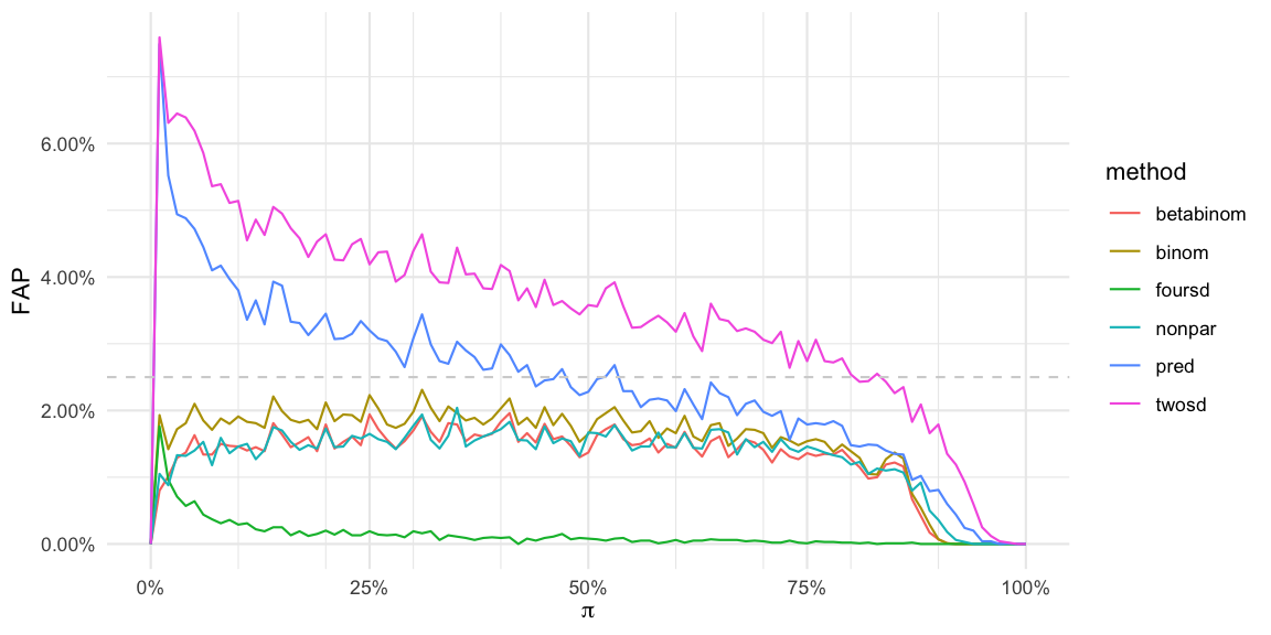
In the figure we see that both the two and four times standard deviation approach (twosd, foursd) as well as the approach based on the 97.5% predictive distribution in a Gaussian setting (pred) have a varying FAP over the range of true proportions: The smaller \(\pi\) the higher the FAP: The FAP can be as high as 7% instead of the nominal 2.5%. When monitoring 145 time points this means that we will on average see \(145\cdot 0.07=10\) false alarms, if the process does not change. This is problematic, because the behaviour of the detection procedure depends on the underlying \(\pi\): the user will get way more false alarm at low \(\pi\)’s than possibly expecting. Altogether, it appears better to use a slightly higher threshold than 2. However, \(k=4\) looks awfully conservative!
All considered procedures dip down to a FAP of 0% for \(\pi\) near 100%, which means no alarms are sounded here. This is related to the fact that if \(U_{t_0}=n_{t_0}\) then, because \(p_{t_0} > U_{t_0}\) is required before an alarm will be sounded, no alarm is possible. Furthermore, both the beta-binomial, the binomial variant and the non-parametric procedure have FAPs slightly lower than the nominal 2.5%. This is again related to the discreteness of the problem: It might not be possible to find an integer limit \(U\) such that the CDF at \(U\) is exactly 97.5%, i.e. usually \(F(q_{0.975})>0.975\). Because we only sound alarms if \(y_{t_0} > U\), i.e. the probability for this to occur is even smaller, namely, \(1-F(q_{0.975}+1)\).
Note that in the above simulation study the binomial and beta-binomial models are in advantage, because the model used to simulate data is identical and closely identical, respectively, to how data are simulated. In order to make the simulation more comprehensive we investigate an additional scenario where the marginal distribution are binomial \(\operatorname{Bin}(25, 0.215)\), but are correlated3. We simulate variables \(y_t^*\) using an \(AR(1)\) process with parameter \(\rho\), \(|\rho| < 1\), i.e. \[ y_t^* | y_{t-1}^* = \rho \cdot y_{t-1}^* + \epsilon_t, \quad t=2,3,\ldots, \] where \(y_1^* \sim N(0,1)\) and \(\epsilon_t \stackrel{\text{iid}}{\sim} N(0,1)\). These latent variables are then marginally back-transformed to standard uniforms \(u_t \sim U(0,1)\) using the probability integral transform and are then transformed using the quantile function of the \(\operatorname{Bin}(25, 0.215)\) distribution, i.e.
qbinom(pnorm(ystar[t]))
Altogether, this corresponds to a Gaussian copula approach for generating correlated random variables with a given marginal distribution. The correlation between the \(y_t\) will not be exactly \(\rho\) due to the discrete nature of the binomial, but will approach \(\rho\) as \(n\) in the binomial becomes large. Figure 3 shows the results for the false alarm probability based on 10,000 Monte Carlo simulations for marginal \(\operatorname{Bin}(25, 0.215)\) distribution and latent \(AR(1)\) one-off-the-diagonal correlation parameter \(\rho\).
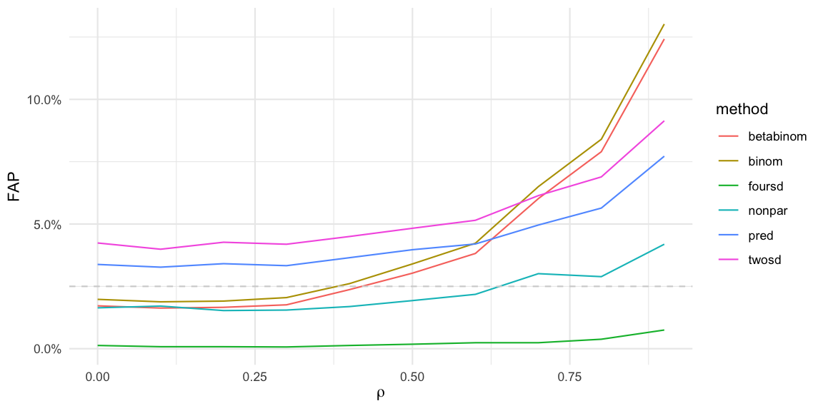 Figure 3: Equivalent of a false alarm probability
by 10,000 Monte Carlo simulation for the algorithms when there is a
correlation \(\rho\) on the latent
scale, but the marginal mean of all observations is \(\pi=0.215\).
Figure 3: Equivalent of a false alarm probability
by 10,000 Monte Carlo simulation for the algorithms when there is a
correlation \(\rho\) on the latent
scale, but the marginal mean of all observations is \(\pi=0.215\).
We see that the binomial and beta binomial approaches sound too many alarms as the correlation increases. Same goes for the two times standard deviation and the predictive approach. The non-parametric approach appears to behave slightly better.
Application
We use the synthetic acute respiratory infection data made available as part of the paper’s SySu Excel tool available for download under a creative common license. In what follows we focus on the time series for the symptom acute respiratory infections. Figure shows the daily proportions 2017-01-01 until 2017-07-20 for all weekdays as vertical bars with the monitoring starting at time point 40. Also shown is the upper threshold \(U_t\) for six methods discussed above.
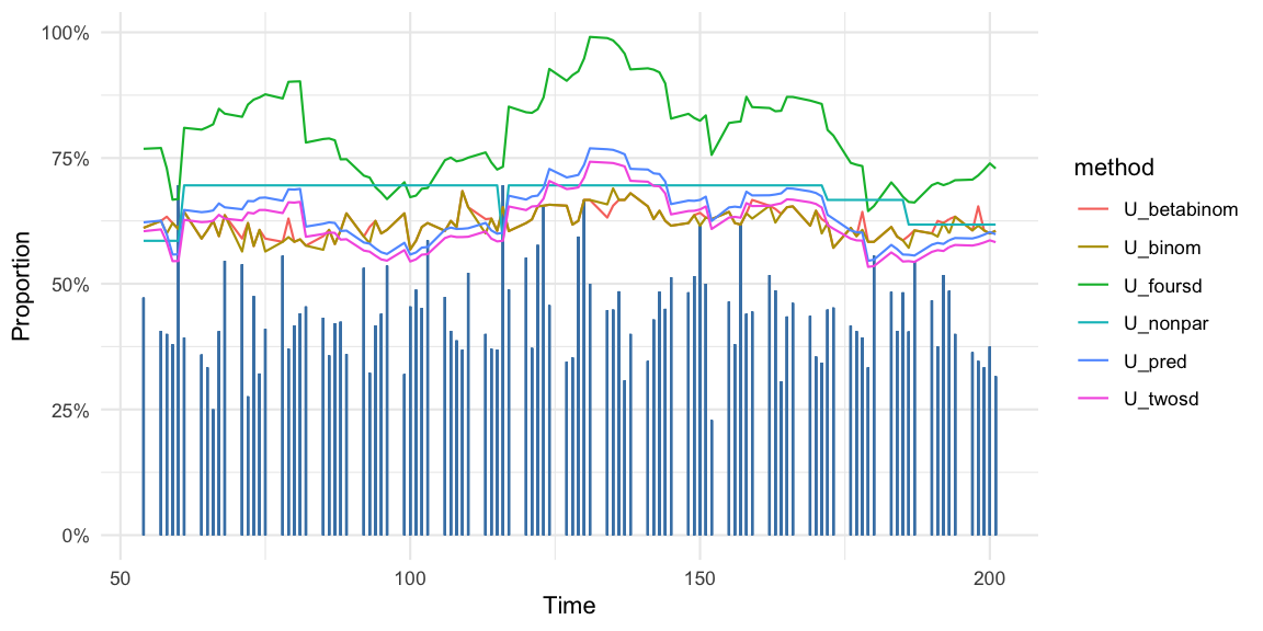
The correlation between \(p_{t}\) and \(p_{t-1}\) in the time series is 0.04, which could be a sign that the synthetic were artificially generated using an independence assumption.
For all algorithms we see the effect on the upper threshold as spikes enter the baseline. In particular the non-parametric method, which uses \(d=39\) baseline values, will only sound an alarm during 39 days after time 60, if the proportion is larger than the \(p_{60} = 69.6\) percent spike.
Discussion
This post discussed how to use statistical process control in order to monitor a proportion within a syndromic surveillance context. The suitability and performance of Gaussian approximations was discussed: It was shown that the false alarm probability for this approach depends on the level of the considered proportion and that auto-correlation also has a substantial impact on the chart. The investigation in this post were done in order to provide the user of such charts with a guidance on how to choose \(k\).
Altogether, a full scientific analysis would need a more comprehensive simulation study and likely access to the real data, but the point of this post was to substantiate that statistical problems need a statistical investigation. From the simulation results in this post it appears more prudent to use \(k>2\), e.g., the upper limit of a 97.5% one-sided prediction interval (\(k\)=2.22) or the upper limit of a 99.5% one-sided prediction interval (\(k\)=3.07). Choosing \(k>2\) is also supported by the fact that Sarma et al. (2018) report that none of the 204 signals generated by the system were subsequently interpreted as an outbreak. Furthermore, a simple fix to avoid confusion could be to chop the upper threshold at 100% in the graphics, i.e. to report \(U_t^* = \max(1, U_t)\) for the Gaussian based procedures. Better would be to use the predictive approach and let the user choose \(\alpha\) and thus give the parameter choice a probabilistic interpretation. However, binomial and beta-binomial based approaches provide more stable results over the full range of \(\pi\) and are guaranteed to respect the \([0,1]\) support. In particular the non-parametric method looks promising despite being even simpler than the proposed k-sd-system. All in all, addressing trends or other type of auto-correlation as well as previous outbreaks in the baseline appears to be important in order to get a more specific syndromic surveillance system - see Sect. 3.4 of Salmon, Schumacher, and Höhle (2016) for how this could look. I invite you to read the Sarma et al. (2018) paper to form your own opinion.
Acknowledgments
The contents of this post were discussed as part of the ht2018 Statistical Consultancy M.Sc. course at the Department of Mathematics, Stockholm University. I thank Jan-Olov Persson, Rolf Sundberg and the students of the course for their comments, remarks and questions.
Conflict of Interest
I have previously worked for the Robert Koch Institute. Some of the co-authors of the Sarma et al. (2018) paper are previous colleagues, which I have published together with.
Literature
The method contains two additional parameters: one being the minimum number of cases needed on a particular day to sound an alarm (low-count protection) and a fixed threshold for the proportion beyond which a signal was always created. For the sake of statistical investigation we shall disregard these two features in the analysis of this post.↩︎
In the paper d=21 was used, but due to many missing values, e.g., due to weekends, the actual number of observations used was on average 15. We therefore use \(d=15\) in the blog post.↩︎
The 21.5% is taken from Table 2 of Sarma et al. (2018) for acute respiratory infections.↩︎