Effective reproduction number estimation

Abstract:

We discuss the estimation with R of the time-varying effective reproduction number during an infectious disease outbreak such as the COVID-19 outbreak. Using a single simulated outbreak we compare the performance of three different estimation methods.

This work is licensed under a Creative Commons Attribution-ShareAlike 4.0 International License. The markdown+Rknitr source code of this blog is available under a GNU General Public License (GPL v3) license from github.

Motivation

A key parameter to know for an infectious disease pathogen like SARS-nCoV-2 is the basic reproduction number, i.e. the expected number of secondary cases per primary case in a completely susceptible population. This quantity and its relation to the susceptible-infectious-recovered (SIR) model was explained in the previous Flatten the COVID-19 curve post. However, as intervention measures are put in place and as a certain proportion of the population gains immunity, interest switches to knowing the time-varying effective reproduction number. This quantity is defined as follows: Consider an individual, who turns infectious on day \(t\). We denote by \(R_e(t)\) the expected number of secondary cases this infectious individual causes. For simplicity we will assume that the timing of being able to infect others and the time of being able to detect this infectivity (e.g. by symptoms or by a test) coincides, i.e. on day \(t\) the above individual will also appear in the incidence time series. The time between symptom onset in the primary case and symptom onset in the secondary case is called the serial interval. The distribution from which the observed serial intervals origin is called the serial interval distribution. Note that this is different from the generation time, which is the time period between exposure of the primary case and exposure of the secondary case. However, since time of exposure is rarely observable, one instead has to use the time series of incident symptom onsets as basis for inference - see also Svensson (2007) for a thorough discussion of the distinction between the generation time and the serial interval. For the sake of simplicity, but slightly against the reality of SARS-nCoV-2, the remainder of this post will not distinguish between the generation time and the serial interval and will also assume that the serial interval is always positive.

The motivation of this blog post is now to show how to estimate the time-varying effective reproduction number \(R_e(t)\) using R - in particular the R package R0 (Obadia, Haneef, and Boëlle 2012). The R code of this post is available from github. We shall consider three estimators from the literature. One of the estimators is used by the German Robert-Koch Institute (RKI). Since 8th of April 2020 the estimate is reported as part of their daily COVID-19 situational reports and is thus discussed by major German news media (e.g. ARD).

Outbreak simulation

We consider a simple growth model and denote by \(y_t\) the expected number of new symptom onsets we observe on day \(t\). Let \((g_1, \ldots, g_M)'\), denote the probability mass function of the serial interval distribution, i.e. \(P(GT=i) = g_i\) for \(i=1,2,\ldots, M\) . The development in the expected number of cases can be described by the homogeneous linear difference equation \[ \begin{align*} y_t = R_e(t-1) g_1 y_{t-1} + \ldots + R_e(t-M) g_M y_{t-M} = \sum_{i=1}^M R_e(t-i) g_i y_{t-i}, \end{align*} \] where \(t=2, 3, \ldots\) and where we on the RHS ignore terms when \(t-M \leq 0\). Furthermore, we fix \(y_1=1\) and conceptually denote by \(t=1\) the 15th of February 2020 in calendar time. To simulate a COVID-19 like outbreak with lockdown type intervention we use \[ \begin{align*} R_e(t) = \left\{ \begin{array}{} 2.5 & \text{if } t \leq \text{2020-03-15} \\ 0.95 & \text{otherwise} \end{array} \right. \end{align*} \]

Serial Interval Distribution

In what follows we shall use a simple discrete serial interval distribution with support on the values 1-7 days. Such a distribution can easily be stated as

GT_pmf <- structure( c(0, 0.1, 0.1, 0.2, 0.2, 0.2, 0.1, 0.1), names=0:7)
GT_obj <- R0::generation.time("empirical", val=GT_pmf)
GT_obj

## Discretized Generation Time distribution
## mean: 4 , sd: 1.732051 
##   0   1   2   3   4   5   6   7 
## 0.0 0.1 0.1 0.2 0.2 0.2 0.1 0.1

Note that the selected PMF of the serial interval has mean 4.00 and is symmetric around its mean.

Outbreak simulation

# Define time varying effective reproduction number
Ret <- function(date) ifelse(date <= as.Date("2020-03-15"), 2.5, 0.95)

# Generate an outbreak (no stochasticity, just the difference equation)
out <- routbreak(n=60, Ret=Ret, GT_obj=GT_obj)
out <- out %>% mutate(ratio = y/lag(y))

We simulate an outbreak using the above difference equation for the selected serial interval distribution starting with one initial case on 2020-02-15. The daily incidence curve of the simulated outbreak looks as follows:

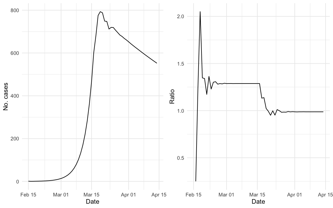
For better visualisation the right hand panel shows a plot of \(q_t = y_{t}/y_{t-1}\). One interesting question is how \(q_t\) is related to \(R_e(t)\).

Wallinga and Teunis (2004)

The method of Wallinga and Teunis (2004) developed as part of the 2003 SARS outbreak is available as function R0::est.R0.TD. It uses a statistical procedure based on the relative likelihood for two cases \(i\) and \(j\) with symptom onset at times \(t_i > t_j\) to be a possible infector-infectee pair. Further methodological details of the method can be found in the paper.

In code:

est_rt_wt <- function(ts, GT_obj) {
  end <- length(ts) - (length(GT_obj$GT)-1)
  R0::est.R0.TD(ts, GT=GT_obj, begin=1, end=end, nsim=1000)
}

Wallinga and Lipsitch (2006)

Wallinga and Lipsitch (2006) discuss the connection between the generation time distribution and the reproduction number. They derive the important relationship that \(R = 1/M(-r)\), where \(r\) is the per-capita growth-rate of the epidemic and \(M(\cdot)\) is the moment generating function of the generation time distribution. As an example, if the generation time distribution is a point-mass distribution with all mass at the value \(G\) then \(M(u) = \exp(u G)\). Two possible estimators for \(R\) in dependence of the generation time would be: \[ \begin{align*} R &= \exp(r \cdot G) & \text{(generation time is a point mass at G)}\\ R &= \left[\sum_{k=1}^\infty \exp(-r \cdot k) \cdot g_k\right]^{-1} & \text{(discrete generation time with PMF } g_1,g_2,\ldots) \end{align*} \]

A simple way to make the above an effective reproduction number estimate is to use a sliding window of half-size \(w\) centered around time \(t\) in order to estimate the growth rate parameter \(r\). For example using a Poisson GLM model of the kind \[ \begin{align*} y_s &\sim \operatorname{Po}(\lambda_s), \text{ with }\\ \log(\lambda_s) &= a + r s, \end{align*} \] where \(s=t-w,\ldots, t+w\). An estimator for \(r\) is then easily extracted together with a confidence interval using a glm approach. In code:

#' Window limited exponential growth rate estimator as in 
#' Wallinga & Lipsitch (2007). 
#'
#' @param ts Time series of incident counts per time interval
#' @param GT_obj PMF of the generation time R0.GT object 
#' @param half_window_width Integer denoting the half-window width

est_rt_exp <- function(ts, GT_obj, half_window_width=3L) {
  # Loop over all time points where the sliding window fits in
  res <- sapply((half_window_width+1):(length(ts)-half_window_width), function(t) {
    # Define the sliding window
    idx <- (t-half_window_width):(t+half_window_width)
    data <- data.frame(Date=1:length(ts), y=as.numeric(ts))
    # Fit a Poisson GLM
    m <- glm( y ~ 1 + Date, family=poisson, data= data  %>% slice(idx))
    # Extract the growth rate 
    r <- as.numeric(coef(m)["Date"])
    
    # Equation 2.9 from Wallinga & Lipsitch
    R <- R.from.r(r, GT_obj)
    return(R)
  })
  names(res) <- names(ts)[(half_window_width+1):(length(ts)-half_window_width)]
  return(res)
}

RKI Method

In a recent report [an der Heiden and Hamouda (2020)]¹ the RKI described their method for computing \(R_e(t)\) as part of the COVID-19 outbreak as follows (p. 13): For a constant generation time of 4 days, one obtains \(R\) as the ratio of new infections in two consecutive time periods each consisting of 4 days. Mathematically, this estimation could be formulated as part of a statistical model: \[ \begin{align*} y_{s+4} \>| \> y_s &\sim \operatorname{Po}(R \cdot y_s), \quad s=1,2,3,4. \end{align*} \] where \(y_1,\ldots, y_4\) are considered as fixed. From this we obtain \(\hat{R}_{RKI}=\sum_{s=1}^4 y_{s+4} / \sum_{s=1}^4 y_{s}\). If we use a GLM to fit the model, we not only get \(\hat{R}\) but also a confidence interval for \(R\) out-of-the box. Somewhat arbitrary, we denote by \(R_e(t)\) the above estimate for \(R\) when \(s=1\) corresponds to time \(t-8\), i.e. we assign the obtained value to the last of the 8 values used in the computation.

In code:

#' RKI R_e(t) estimator with generation time GT (default GT=4). Note: The time t
#' is assigned to the last day in the blocks of cases on [t,t+1,t+2, t+3] vs.
#' [t+4,t+5,t+6, t+7], i.e. s=t-8 (c.f. p. 14 of 2020-04-24 version of the RKI paper)
#' @param ts - Vector of integer values containing the time series of incident cases
#' @param GT - PMF of the generation time is a fixed point mass at the value GT.

est_rt_rki_last <- function(ts, GT=4L) {
  # Sanity check
  if (!is.integer(GT) | !(GT>0)) stop("GT has to be postive integer.")
  # Estimate, if s=1 is t-7
  res <- sapply( (2*GT):length(ts), function(t) {
    sum(ts[t-(0:(GT-1))]) / sum(ts[t-2*GT+1:GT])
  })
  names(res) <- names(ts)[(2*GT):length(ts)]
  return(res)
}

Basically, the method appears to be the Wallinga and Lipsitch (2006) approach using a point mass generation time distribution, but with a slightly different timing of the sliding windows. However, since no references were given in the RKI publication, I got curious: what happens for this approach when the generation time distribution is not a point mass at \(G\)? What happens if the mean generation time is not an integer? 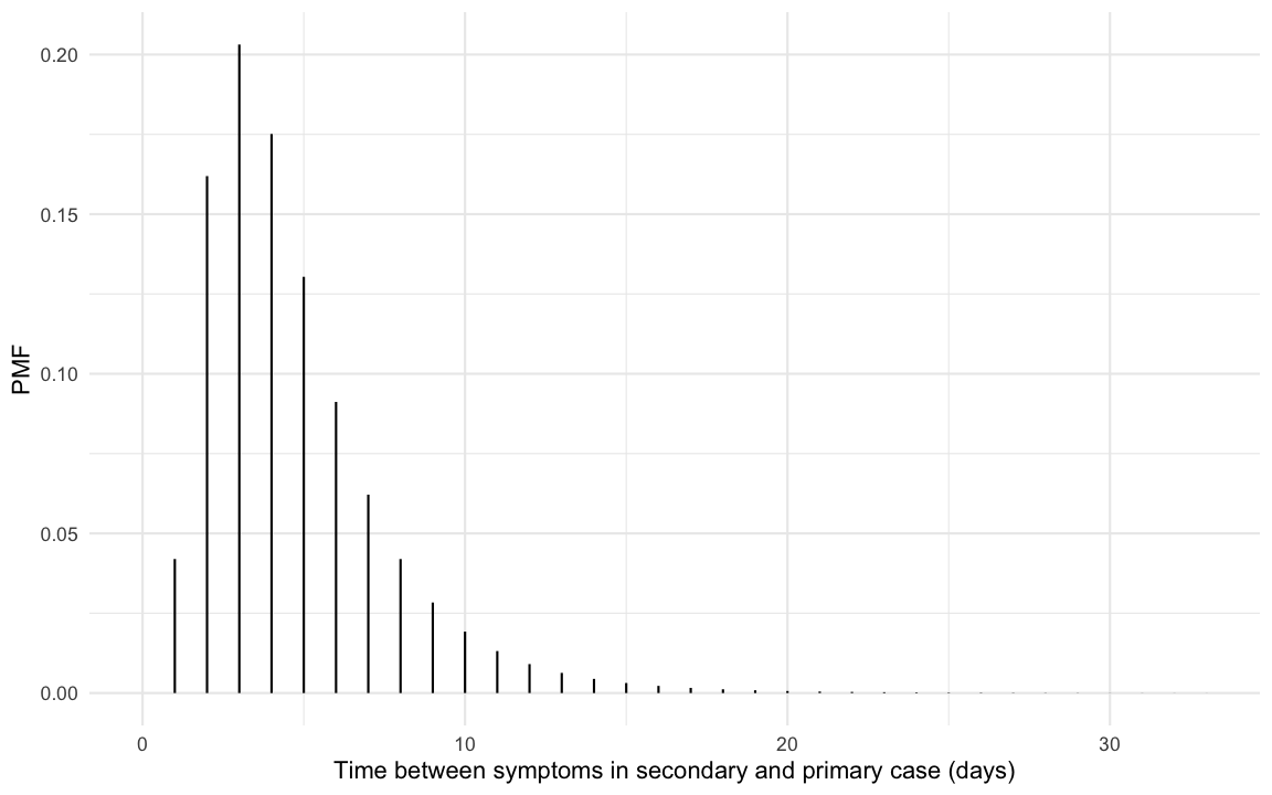That these are not purely hypothetical question is underlined by the fact that (nishiura_serial_2020?) find a serial interval distribution with mean 4.7 days and standard deviation 2.9 as the most suitable fit to data from 28 COVID-19 infector-infectee pairs. Such a serial interval distribution has the following shape:

The Comparison

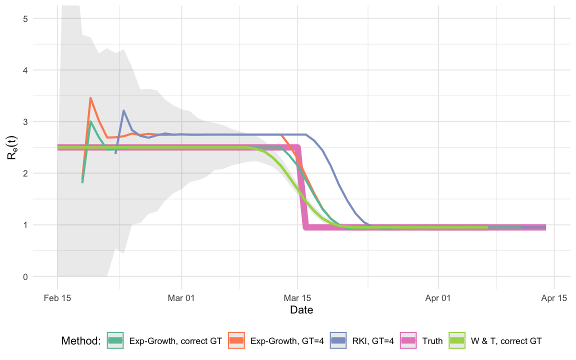
The aim of this post is thus to compare the performance of the RKI estimator with both the Wallinga and Teunis (2004) and the Wallinga and Lipsitch (2006) estimators for the single outbreak simulated in this post. Results do, however, generalize to other configurations.

We compute and plot of the \(R_e(t)\) estimates:

# RKI method as specified in 2020-04-24 version of the article
rt_rki_last <- est_rt_rki_last(out$y  %>% setNames(out$Date), GT=4L)

# Exponential growth with discrete Laplace transform of a GT \equiv = 4 distribution
rt_exp2 <- est_rt_exp( out$y %>% setNames(out$Date), GT_obj=R0::generation.time("empirical", c(0,0,0,0,1,0,0,0)), half_window_width=3)

# Exponential growth with discrete Laplace transform of the correct GT distribution
rt_exp <- est_rt_exp( out$y %>% setNames(out$Date), GT_obj=GT_obj, half_window_width=3)

# Wallinga Teunis approach with correct GT distribution
rt_wt <- est_rt_wt( out$y, GT=GT_obj)

# Data frame with the true values
Ret_true <- data.frame(Date=out$Date) %>% mutate(R_hat=Ret(Date), Method="Truth")

The shaded area indicates the pointwise confidence intervals of the Wallinga and Teunis (2004) method. To make the results of the graph more explicit, we take a look at 3 time points in the beginning of the outbreak:

##         Date W & T, correct GT RKI, GT=4 Truth Exp-G, correct GT
## 1 2020-03-11          2.418862  2.748119   2.5          2.499998
## 2 2020-03-12          2.303251  2.748070   2.5          2.500003
## 3 2020-03-13          2.140055  2.748073   2.5          2.500000

and 3 time points at the end of the outbreak:

##         Date W & T, correct GT RKI, GT=4 Truth Exp-G, correct GT
## 1 2020-04-05              0.95 0.9499707  0.95         0.9502002
## 2 2020-04-06              0.95 0.9500350  0.95         0.9501288
## 3 2020-04-07              0.95 0.9499612  0.95         0.9500405

One observes that the RKI method has a bias in this situation. To some extent this is not surprising, because both the W & T method as well as the exponential growth model use the correct generation time distribution, whereas the RKI method and the exponential growth with point mass distribution use an incorrect serial interval distribution. In practice “the correct” serial interval distribution would not be available – only an estimate. However, one could reflect estimation uncertainty through additional bootstrapping of the two more advanced methods. A more thorough investigation of the methods would of course also have to investigate the effect of misspecification for the W & T (2004) method or the exponential growth approach. The point is, however, that the RKI method as stated in the report is not able to handle a non-point-mass generation time distribution, which does seem necessary. There might be other reasons for choosing such a simplified distribution, but from a statistical point of view it seems like the estimator could be improved.

Instantaneous reproduction number

Update 2020-04-22: Based on recent discussions, I’m adding an additional reproduction number estimator, i.e. the instantaneous reproduction number as defined in Cori et al. (2013). This quantitity is different from the effective reproduction number, because it compares the number of new infections on day \(t\) with the infection pressure from the days prior to \(t\), i.e.

\[ \hat{R}(t) = \frac{y_t}{\sum_{s=1}^{t} g_{s} \cdot y_{t-s}} \]

It can be interpreted as the average number of secondary cases that each symptomatic individual at time \(t\) would infect, if the conditions remained as they were at time \(t\).

Opposite to the forward looking approach of Wallinga and Teunis (2004), this estimator is defined backwards in time. As illustrated by this comment to a JAMA paper by Lipsitch et al., the definition of timing of \(R(t)\) can make a big difference when comparing it with intervention measures. The instantaneous reproduction number estimator is implemented in the EpiEstim package (Cori et al. 2013). For our small simulation and without any smoothing window for the instantaneous estimator we obtain

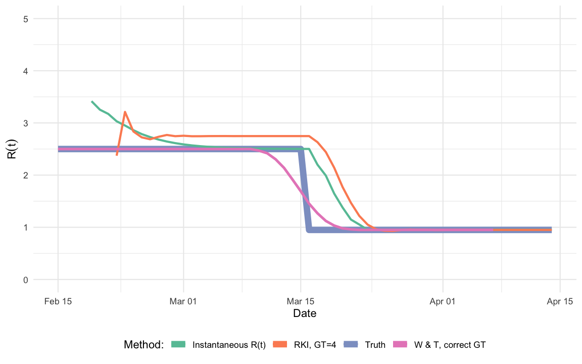
One observes that the change of the estimate in timing corresponds to the intervention, but it takes time to adjust to the new situation and, hence, provides too high values reproduction number values for some days after the intervention, which is the point of Lipsitch et al.. The plot shows how difficult it is to use reproduction number estimates to assess interventions, where the change is abrupt and at a time scale shorter than the serial interval. Furthermore, since the RKI method is assigned to the last time point of the two 4-blocks compared, it appears in interpretation to be closer to the instantenous reproduction number.

At this point it is good to remember why one started to consider the effective reproduction number in the first place. That is, as a real-time (i.e. with interventions and immunity) extension of the basic reproduction number \(R_0\). To me this definition is inherently forward in time.

Discussion

In this post we showed how to compute the effective reproduction number in R using both own implementations and the R0 package. We illustrated this with data from a hypothetical outbreak. An important message is that there is a mathematical relationship between the daily growth factor and the reproduction number - this relationship is governed by the generation time distribution.

In the present analysis the RKI method, which basically is identical to the approach of inserting the point mass distribution into the formula of Wallinga and Lipsitch (2006), showed a bias when the generation time had the anticipated mean, but had a standard deviation larger than zero. The bias is more pronounced when \(R_e(t)\) is further away from 1. However, once the lockdown is gradually lifted, \(R_e(t)\) is likely to raise again making this potentially a relevant bias. The exponential growth approach using the moment generating function of the (discretized) best estimate of the serial interval distribution, can be realized with any statistics package and is computationally fast. Further algorithmic improvements such as Wallinga and Teunis (2004) are readily available in R.

A nice site, which computes time varying reproduction rates for many countries in the world is Temporal variation in transmission during the COVID-19 outbreak by the LSHTM.

Literature