How to Win a Game (or More) of Super Six
Abstract:
We use simulation to analyse the family dicing game “Super Six”. In particular we show that the person starting the game has a very high chance of winning the game. Furthermore, a robust strategy to play during the game is to keep throwing the dice regardless of the number of free pits. In a mixed strategy landscape with more than two players this seems to do better than a strategy extrapolated from the analytically derived optimal strategy for the two player case.
 This work is licensed under a Creative Commons
Attribution-ShareAlike 4.0 International License. The R-markdown
source code of this blog is available under a GNU General Public
License (GPL v3) license from GitHub.
This work is licensed under a Creative Commons
Attribution-ShareAlike 4.0 International License. The R-markdown
source code of this blog is available under a GNU General Public
License (GPL v3) license from GitHub.
Introduction
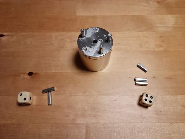
Super Six is a dice game which can be played at all ages. It consists of a container where the lid has 5 pits (labelled 1-5) and one hole (labelled 6). Furthermore, each player gets a predetermined number of sticks and a dice (see Fig.1). If a stick is put into pit 6 (the hole) it falls into container and stays there.
The rules of the games are as follows: The sticks are distributed among the players so that each player has exactly the same number of sticks (say: 4). Each player throws the dice in turn going round in clockwise direction. If a player throws a number and the corresponding pit is empty, then he/she can insert one of his/her sticks into it. If the pit is already occupied, however, then he/she must take the stick and and add it to his/her own pile of sticks. The number 6 is a “lucky throw”. With a 6, one can always place a stick into the hole labelled No. 6 and it stays there. Note: During the first round, each player is only allowed to throw the dice once. From the second round on, each player can throw the dice as often as desired, provided that one always managed to hit an empty pit. As soon as one throws the number of an occupied pit, one must take the stick that is located there and it is then the next players turn. Each player most throw the dice at least once per round, but after the first throw he/she can decide to stop throwing at any time in that round (that is also before hitting an occupied pit). Once a player has no sticks left, the game is over and he/she is the winner. This YouTube video by Rüdiger Jehn shows a exemplary game play of Super Six.
Empirical experience from playing a lot of Super 6 with the kids raises the question if the game is really fair: Does the player starting the game have a winning advantage? Furthermore, interest is in the optimal strategy to play: Should one always continue to throw the dice until one hits an occupied pit or should one stop playing once there are only \(x\) out of the 5 pits free (with \(x\) being either 1 or 2)? In what follows we shall use simulation to get an approximate answer to these questions in a realistic environment with different players following different strategies. For a two player situation analytic results exist (Jehn 2021).
Simulating Super 6
The file super6.R
contains a function simulate_super6 with arguments
players_strategy and sticks to simulate a game
of Super 6 for \(n\)=length(players_strategy)
players each initially having sticks number of sticks. The
named list players_strategy contains each player’s strategy
as a tibble, mapping the number of free pits
(i.e. 0,1,2,3,4,5) to a probability to continue throwing the dice. If
this probability is either 0 or 1 then we have a deterministic strategy.
As an example the always strategy describes a behaviour
where one keeps throwing the dice independent of the number of free
pits:
(always <- tibble(filled_holes=0:5, continue_prob=1))## # A tibble: 6 × 2
## filled_holes continue_prob
## <int> <dbl>
## 1 0 1
## 2 1 1
## 3 2 1
## 4 3 1
## 5 4 1
## 6 5 1As an example: To simulate a single game of Super 6 with three players, A, B and C, each playing the “always” strategy with initially 4 sticks we call
h <- simulate_super6(list(A=always, B=always, C=always), sticks=4)The resulting trajectory of state and actions of the game are returned by the function:
| round | player | turn | dice | hole.1 | hole.2 | hole.3 | hole.4 | hole.5 | hole.6 | sticks.A | sticks.B | sticks.C | decision |
|---|---|---|---|---|---|---|---|---|---|---|---|---|---|
| 1 | C | 1 | 6 | 0 | 0 | 0 | 0 | 0 | 1 | 4 | 4 | 3 | stop turn |
| 1 | A | 1 | 3 | 0 | 0 | 1 | 0 | 0 | 1 | 3 | 4 | 3 | stop turn |
| 1 | B | 1 | 2 | 0 | 1 | 1 | 0 | 0 | 1 | 3 | 3 | 3 | stop turn |
| 2 | C | 1 | 2 | 0 | 0 | 1 | 0 | 0 | 1 | 3 | 3 | 4 | lost turn |
| 2 | A | 1 | 6 | 0 | 0 | 1 | 0 | 0 | 2 | 2 | 3 | 4 | continue turn |
| 2 | A | 2 | 3 | 0 | 0 | 0 | 0 | 0 | 2 | 3 | 3 | 4 | lost turn |
| 2 | B | 1 | 5 | 0 | 0 | 0 | 0 | 1 | 2 | 3 | 2 | 4 | continue turn |
| 2 | B | 2 | 4 | 0 | 0 | 0 | 1 | 1 | 2 | 3 | 1 | 4 | continue turn |
| 2 | B | 3 | 6 | 0 | 0 | 0 | 1 | 1 | 3 | 3 | 0 | 4 | game over |
Note that in the above game the player to start is randomly selected.
The players then each take turns in the pre-determined order. The order
of the rows in the table corresponds to the sequence of actions in the
game. The column turn is a counter indicating how many
times the player has thrown the dice during his/her round. The columns
hole.1-hole.5 are binary indicators whether
the respective pit is currently filled with a stick (FALSE=0, TRUE=1).
Finally, a column counts for each player the current number of remaining
sticks (initially equal to 4). The last column, decision
contains information about the player’s action and its consequences.
Here, “stop turn” is a forced decision in round 1, because each player
can only throw the dice once in round 1. Furthermore, “lost turn”
indicates the situation that the pit indicated by the dice throw was
already occupied and “continue turn” means that the player based on
his/her strategy decided to throw again. Finally, “game over” means that
one player reduced their number of sticks to zero and the game thus
ends. The winner of the shown game shown is B.
Analysis
We can use the above simulation function to analyse different strategies for games with 4 initial sticks. Consider the four additional strategies:
go50 <- tibble( filled_holes=0:5,   continue_prob=1*(filled_holes<=3))
go67 <- tibble( filled_holes=0:5,   continue_prob=1*(filled_holes<=4))
random <- tibble( filled_holes=0:5, continue_prob=0.5)
random2 <- tibble(filled_holes=0:5, continue_prob=c(1,1,1,1,0.5,0.25))
Let’s assume that Agneta is playing the always strategy
and that Bertil, Cecilia, Dagmar and Emil each are playing one of the
four other strategies.
player_list <- list(Agneta= always,
                    Birger= go50,
                    Carin=  go67,
                    Dagmar= random,
                    Emil=   random2)
player_names <- names(player_list)
We now consider all possible matches of these players. This can be games ranging from just 2 of the players to all 5 of them.
n_players <- 2L:length(player_names)
matches <- map(n_players, function(m) {
  utils::combn(player_names, m=m, simplify=FALSE)
}) %>% setNames(n_players)
n_combos <- map(matches, length)
n_combos %>% unlist()
## 2 3 4 5
## 10 10 5 1To ensure that the we consider an equal amount of games for every
number of players, we simulate n_games games for each
number of players (2-5). The games to play are then distributed equal
among the different pairings with that number of players. For this
reason, n_games has to be divisible by 5 and 10.
n_games <- 10000

# Parallelize analysis using the future-verse
plan(multisession, workers = 4)

# Play the games
all_games <- future_map2(matches, n_combos,  function(names, combos) {
  map(names, ~ {
    the_players_strategy <- player_list[.x]
    # Divide the n_games equal among the possible combinations
    n_games_each_combo <- n_games / combos
    map(seq_len(n_games_each_combo), ~
          simulate_super6(players_strategy=the_players_strategy, sticks=4)
    )
  }) %>% setNames(map(names, ~ str_c(.x, collapse="-")))
}, .options=furrr_options(seed=TRUE))
This provides a nested list structure, where the top-most level contains the number of players of the game, the 2nd level contains the name of the participating players and the 3rd level the recordings of every game played of the respective player combination (organised as a tibble). The recordings/history of each game is organised as a data frame with columns closely related to the above game description. As an example, a total of
all_games[["3"]][["Agneta-Birger-Carin"]] %>% length()## [1] 1000games (=10000/10) are played between the players Agneta, Birger and Carin.
We now use this nested list structure of simulated games to answer our questions of interest. The traversing of the list is done by purrr. As an example we determine the total number of games as follows:
(n_total_games <- map(all_games, ~ map(.x, length)) %>% unlist() %>% sum())## [1] 40000Beginner is Winner?
We now investigate the probability to win the starting player. Let
h denote the tibble describing the history of a game (such
as shown above). We will write a function, which given the history of a
game returns the player name who won the game.
winner <- function(h) {
  h %>% slice_tail(n=1) %>% pull(player)
}

## Test the function on the above shown trajectory
winner(h)
## [1] "B"We can use the function to determine the probability that the player starting the game also becomes the winner of the game. To take into account a possible dependence on the number of players we shall stratify our analysis by the number of players in the game.
games_summary <- map2_df(all_games, n_players, function(games, players) {
  map_df(games, ~map_df(.x, ~ tibble(n_players=as.numeric(players),
                        beginner=.x %>% slice_head(n=1) %>% pull(player),
                          winner=.x %>% slice_tail(n=1) %>% pull(player))))
})

tab <- games_summary %>% group_by(n_players) %>%
  summarise(p_initial_winner=mean(beginner==winner)) %>%
  mutate(p_random = 1/n_players,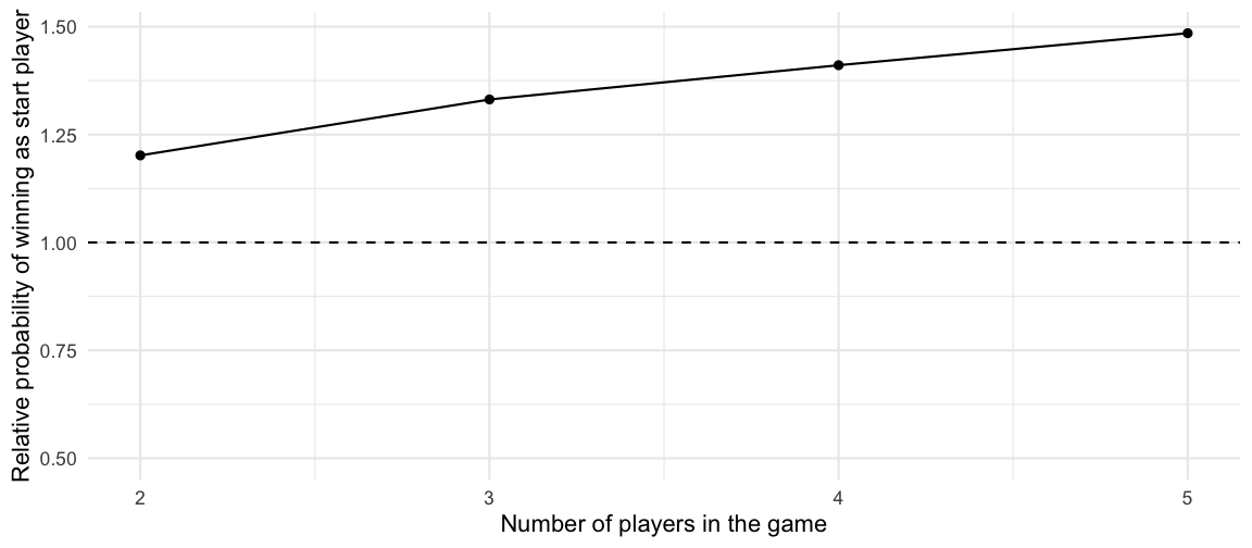
favor_factor = p_initial_winner / p_random) | n_players | p_initial_winner | p_random | favor_factor |
|---|---|---|---|
| 2 | 0.6009 | 0.5000000 | 1.2018 |
| 3 | 0.4438 | 0.3333333 | 1.3314 |
| 4 | 0.3527 | 0.2500000 | 1.4108 |
| 5 | 0.2970 | 0.2000000 | 1.4850 |
The empirical probability that the initial player wins is always
higher than the probability \(1/n\)
that one of the \(n\) players in the
game wins at random. The larger the number of players the bigger the
relative advantage of beginning seems. Note that our analysis averages
over the all strategies so it also contains start players using an
otherwise sub-optimal playing strategy. This might bias the analysis
slightly, but a small sensitivity analysis letting all 5 players play
the always strategy, showed that results did not change
substantially.
Best strategy
We can now compute for each player (i.e. strategy) the number of wins out of the 40000 games:
(league_table <- map(all_games, ~ map(.x, ~ map(.x, winner))) %>%
  unlist() %>%
  as_tibble() %>%
  rename(player = value) %>%
  group_by(player) %>%
  summarise(wins=n()) %>%
  arrange(desc(wins)))
## # A tibble: 5 × 2
## player wins
## <chr> <int>
## 1 Birger 8800
## 2 Carin 8593
## 3 Emil 8520
## 4 Agneta 8419
## 5 Dagmar 5668This shows that the always strategy appears to do best
among those strategies investigated. It is no surprise that the worst
strategy is the purely random strategy random.
Discussion
We analysed aspects of how to win a game (or more) of Super Six. Important factors for winning in a multi-player mixed strategy landscape are
- To start the game
- To keep throwing the dice
A little surprising is that the best strategy (among those investigated) is to keep throwing the dice regardless of the number of free pits. The optimal strategy may in part depend on how the other players play, but our conclusions appear sufficiently robust, because the simulation study investigated a mixed strategy player field with two to five players. A limitation of our analysis is that we only considered games where each player initially holds 4 sticks.
It is worth pointing out that the best strategy we found is not optimal. As an example, Jehn (2021) analytically finds the optimal strategy for the \(n=2\) player situation. It depends on the number of sticks left in the game and the number of sticks each player has. In most cases the strategy stops if more than 3 pits are occupied – see Appendix 1 for details. This dependence on the other player’s hand is likely to carry forward to the \(n>2\) player situation. However, analytic results for \(n>2\) will be extremely difficult to obtain, but it makes intuitive sense to be more aggressive when there are more players, because there are more contestants for the win.
Did the game developers realize that the start player has such a high probability of winning the game? It seems advisable to accompany game development by simulations and mathematical calculations at the design stage. In practice, one should randomize the start player to enhance fairness.
Final note: This will be the last post of Theory Meets Practice Blog in its current form. As of Jan 2023 I am working as full professor in Statistics and Data Science at the University of Greifswald, Germany. For both technical and time reasons a new setup is thus needed.
Appendix 1
The work of Jehn (2021) shows the derivation of the optimal strategies encoded in A345383 for a game with 2 players and a situation where \(i\) pits occupied, the first player (our player of interest) has \(j\) sticks in hand and the second player has \(k\) sticks. This state is denoted as \(i/j/k\). For example \(2/1/1\) denotes the situation where there are 2 pits occupied in the lid and each player has one stick.
A small helper function gives all states where a continue vs. stop choice needs to be made. It is assumed that if there are no sticks in the lid, we always continue:
#' Find all situations where a continue vs. stop choice is to be made
#' for player 1.
#'
#' See Jehn (2021), https://arxiv.org/pdf/2109.10700.pdf, for details.
#'
#' @param n Total number of sticks currently (i+j+k)
#' @return A vector of strings describing the situations in i/j/k notation
#' where i is the number of occupied pits in the lid, j is the number of
#' sticks player 1 has and k is the number of sticks player 2 has. Note
#' i+j+k = n
#'
situations <- function(n) {
  res <- NULL
  # Sticks in the Lid
  for (i in min(n,5):1) {
    # Sticks Player 1
    for (j in n:1) {
      # Sticks Player 2
      k <- n - i - j
      # Don't consider impossible situations or situations without a choice
      if (k>0  & !(i==0 & j==k)) {
        res <- append(res, str_c(c(i,j,k), collapse="/"))
      }
    }
  }
  return(res)
}

# All situations when there are 7 sticks left in the game
situations(n=7)
## [1] "5/1/1" "4/2/1" "4/1/2" "3/3/1" "3/2/2" "3/1/3" "2/4/1" "2/3/2" "2/2/3" "2/1/4" "1/5/1" "1/4/2" "1/3/3" "1/2/4" "1/1/5"The optimal strategy is encoded in binary and converted to base 10 in the sequence A345383. We write a small R extractor to display the optimal strategy in more readable form:
## Handle the large integers using the GMP library
suppressPackageStartupMessages(library(gmp))

#' Encodes [A345383](https://oeis.org/A345383)
#'
#' @param n Number of sticks
#' @returns a(n) from A345383
#'
a <- function(n) {
  a <- as.bigz(c(0, 0, 1, 7, 63, 1023, 32760, 1048544, 33554304, 1073741312, 34359736320, 1099511619584, 35184370221056, 1125899873681408, 36028796752101376))
  if (n>=1 & n<=15) return(a[n]) else return(NA)
}

#' Convert a strategy encoded as a 0/1 string to a vector of Booleans
#' @param s The strategy as a string of 0 and 1's
#' @return As a vector
#' @examples
#' int_strategy_to_vec("0011")
int_strategy_to_vec <- function(s) {
  str_split_1(as.character(s, b=2), pattern="") %>% as.integer()
}

#' Show the optimal stragegy for all situations with n sticks
optimal_strategy <- function(n) {
  # Make a tibble representing the optimal strategy
  tibble(situation= situations(n),
         continue = rev(int_strategy_to_vec(a(n))))
}

optimal_strategy(n=7) %>% print(n=Inf)
## # A tibble: 15 × 2
## situation continue
## <chr> <int>
## 1 5/1/1 0
## 2 4/2/1 0
## 3 4/1/2 0
## 4 3/3/1 1
## 5 3/2/2 1
## 6 3/1/3 1
## 7 2/4/1 1
## 8 2/3/2 1
## 9 2/2/3 1
## 10 2/1/4 1
## 11 1/5/1 1
## 12 1/4/2 1
## 13 1/3/3 1
## 14 1/2/4 1
## 15 1/1/5 1We observe that for situations with 7 sticks we continue to play as long as only 1-3 pits are filled. If 4 or 5 pits are filled, we don’t continue. However, in other settings with different number of sticks left, the optimal strategy can be different. As an example, if there 6 sticks left, the optimal strategy is
## # A tibble: 10 × 2
##    situation continue
##    <chr>        <int>
##  1 4/1/1            1
##  2 3/2/1            1
##  3 3/1/2            1
##  4 2/3/1            1
##  5 2/2/2            1
##  6 2/1/3            1
##  7 1/4/1            1
##  8 1/3/2            1
##  9 1/2/3            1
## 10 1/1/4            1
which -opposite to the 7 sticks left situation- continues in the 4 pits filled situation, if each player has only one stick left (4/1/1).
Finally, we implement a function, which implements Jehn’s optimal
strategy in a way, which can be used by the simulation function
simulate_super6():
#' Jehn's optimal strategy for two players
#'
#' @param player_idx Index of the player in the state_players variable (see simulate_super6 function)
#' @param filled_holes Number of pits filled
#' @param state_players Vector of length equal to the number of players containing the number of sticks each player has left
#' @return A numeric corresponding to the probability to continue
#'
jehn <- function(player_idx, filled_holes, state_players) {
  # Some summaries
  sticks_left <- filled_holes + sum(state_players)
  my_sticks <- state_players[player_idx]
  other_sticks <- state_players[-player_idx]

  #Strategy for basic cases
  if (filled_holes <= 2) return(1)
  if (filled_holes == 5) return(0)
  #Complicated part of the strategy
  s_best <- optimal_strategy(n=sticks_left)
  state <- str_c(filled_holes, my_sticks, other_sticks, sep="/")
  action <- s_best %>% filter(situation == state) %>%
    pull(continue)

  # Check if output fails (this should not happen).
  if (length(action) == 0) { browser()}
  if (!is.numeric(action)) { browser()}

  # Done
  return(action)
}
This allows us to test, if there is a winning advantage, despite both players playing the optimal strategy (see source code for details).
## # A tibble: 1 × 1
##   p_win_beginner
##            <dbl>
## 1          0.596
The answer is thus: Yes! In 60% of the games the starting player
wins. Thus, the winning advantage of the beginner in the \(n=2\) scenario remains even when both
players use the jehn optimal winning strategy.