Guess My Name with Decision Trees
Abstract:
We use classification trees to determine the optimal sequence of questions to ask in the game “Guess my name” (Mini Logix series from Djeco). Aim of the game is to identify wich person, out of 16 possible, the opponent is. Clasification trees and optimal sequential decision making in this case have strong similarities with cross-entropy of the class distribution working as a common metric for quantifying information gain.
 This work is licensed under a Creative Commons
Attribution-ShareAlike 4.0 International License. The R-markdown
source code of this blog is available under a GNU General Public
License (GPL v3) license from GitHub.
This work is licensed under a Creative Commons
Attribution-ShareAlike 4.0 International License. The R-markdown
source code of this blog is available under a GNU General Public
License (GPL v3) license from GitHub.
Introduction
As a mathmatician you do not play logic games for fun, you play to win. So when playing “Guess my name” (Mini Logix series from Djeco), where the task is to ask your opponent a series of questions in order to identify which of 16 picture characters they are, you want to devise an optimal sequence of questions in order to determine your opponent’s choice. Given a catalogue of possible questions, we use classification trees to find the optimal sequence of questions to ask.
The game goes as follows: Each player gets a card with pictures of 16 persons. Each player selects a person of the 16 she wants to be and writes the name of this person on their card.

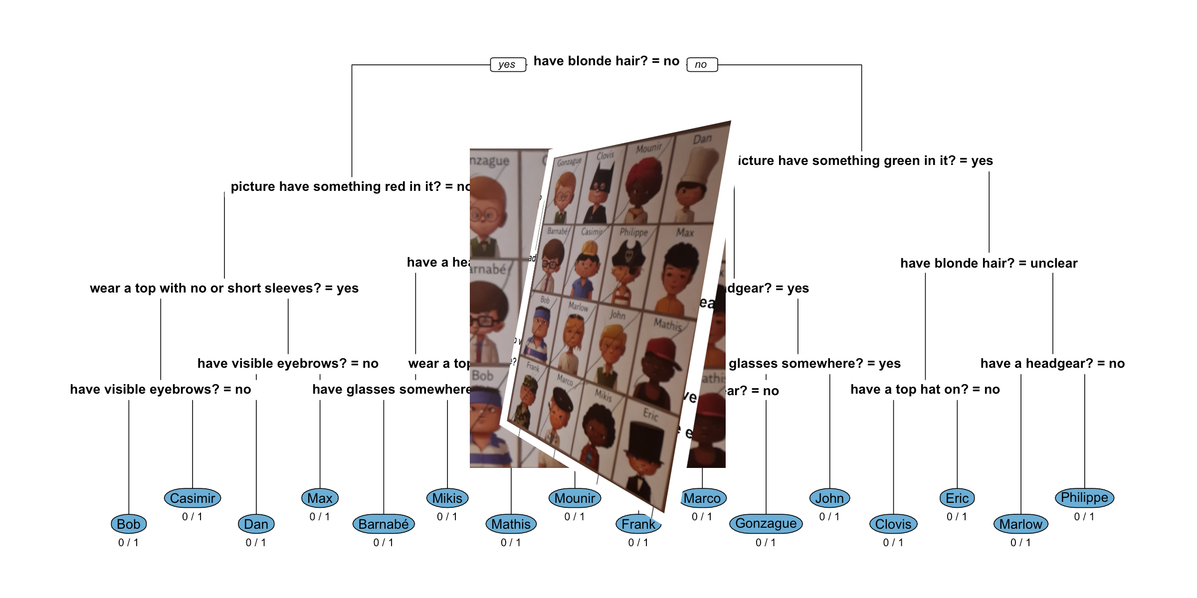
Figure 1: Exemplary game card of the “Guess my name” game, Mini Logix series, Djeco, during gameplay.
The players then take turns to ask the opponent one question about their person, for example you could ask Does your person have glasses? or Is your person wearing a chef’s hat?“. Based on the answer (possible answers are: yes or no) you sequentially rule out more and more persons on the card until you are ready to guess who the other person is. The first player to correctly identify the opponent’s person wins. Note that only questions about the picture of the person are allowed. In what follows, we shall assume that a third answer cateogry”unclear” is also possible, because some questions like does your person have blonde hair can not be answered when the hair is not visible on the picture (see for example the picture of Clovis).
The aim is now to devise a series of questions whick as quickly as possible can narrow our set of candidate persons down to 1 person. When only yes or no answers are possible, in the optimal case, each question reduces the set of possible persons by a factor 2. Hence, \(2^x = 16 \Leftrightarrow x = \log_{2}(16) = 4\) (well chosen) questions are needed to reduce the set of candidates from 16 to 1. However, it might not be possible to find a sequence of such optimal questions, because (given the previous set of questions) the next question might not split the remaining pool of candidates in two sets of equal cardinality. As a more hands-on approach we formulate the task as follows: given a set of questions, where we for each of the 16 persons know the answer to, which questions and in what sequence should we ask them in order to correctly identity the opponent’s person.
Methods
Question Catalogue
To begin with we develop a set of questions and encode the answer of each of the 16 persons to the question as yes, no or unclear Below we show an exemplary question catalogue consisting of 12 together with the answers for 8 out of the 16 persons (full data for all 16 here). One can compare the answers with the picture of the above shown game card.
| Question: Does the person | Gonzague | Clovis | Mounir | Dan | Barnabé | Casimir | Philippe | Max |
|---|---|---|---|---|---|---|---|---|
| have a headgear? | no | yes | yes | yes | no | yes | yes | yes |
| have glasses somewhere? | yes | no | no | no | yes | no | no | no |
| have a brush behind the ear? | no | no | no | no | no | no | no | no |
| have blonde hair? | yes | unclear | no | no | no | no | yes | no |
| wear a top with no or short sleeves? | no | no | no | no | no | yes | yes | no |
| have visible eyebrows? | yes | no | yes | no | yes | yes | no | yes |
| picture have something red in it? | yes | no | yes | no | yes | no | yes | no |
| have a top hat on? | no | no | no | no | no | no | no | no |
| picture have something green in it? | yes | no | no | no | no | no | no | no |
| have blue eyes? | yes | no | no | no | no | no | yes | no |
| have a chef’s hat on? | no | no | no | yes | no | no | no | no |
| have a V-collar? | no | yes | no | no | yes | yes | no | no |
Decision Trees as Classification Trees
We use classification trees to represent the sequence of questions to ask. Our goal is to correctly identify the person at the end of the sequence, hence, each leave node should assign the correct person with 100% probability. This is somewhat opposite to traditional classification trees, which inspired by Occam’s razor are kept small and thus accept a certain misclassification rate on the training data in order to generalize well to out-of-sample data.
We address this tweak by working with saturated trees (i.e. no
pruning). Furthermore, we need to shape the questions s.t. they space of
answers allows for a correct partitioning of all 16 persons. For ease of
exposition we assume that each of the 16 persons is equally likely to be
chosen by your opponent, i.e. the prior probability for each person is
1/16. The appendix “Technical Details” contains information about how
the tree is grown. In R, classification trees can be fitted using the
function rpart::rpart(). We configure the function such
that a saturated tree is grown, if this possible from the question
catalogue. Since training and test data in our case are identical we
want a tree which fits as good as possible on the training data.
Results
We transpose the question catalogue in order to bring the data into a shape with columns being the features and one row per person.
# Tranpose data to a tibble allowing a fit
persons <- questions %>%
  pivot_longer(-`Question: Does the person`, names_to="Person") %>%
  pivot_wider(id_cols = Person, names_from=`Question: Does the person`,
                                values_from=value) %>%
  mutate(across(everything(), factor))
head(persons)
## # A tibble: 6 × 13
## Person `have a headgear?` `have glasses somewhere?` have a brush behind the ea…¹ `have blonde hair?` wear a top with no o…² have visible eyebrow…³
## <fct> <fct> <fct> <fct> <fct> <fct> <fct>
## 1 Gonzague no yes no yes no yes
## 2 Clovis yes no no unclear no no
## 3 Mounir yes no no no no yes
## 4 Dan yes no no no no no
## 5 Barnabé no yes no no no yes
## 6 Casimir yes no no no yes yes
## # ℹ abbreviated names: ¹`have a brush behind the ear?`, ²`wear a top with no or short sleeves?`, ³`have visible eyebrows?`
## # ℹ 6 more variables: `picture have something red in it?` <fct>, `have a top hat on?` <fct>, `picture have something green in it?` <fct>,
## # `have blue eyes?` <fct>, `have a chef's hat on?` <fct>, `have a V-collar?` <fct>This format of the data can then be used with
rpart::rpart().
# Fit tree using rpart
# Make sure we get a saturated tree
tree <- rpart(formula = Person ~ ., data = persons,
              method="class",
              parms=list(split="information"),
              control=rpart.control(minbucket=0, xval=0, cp = -1))
The resulting decision tree is illustrated below. We start at the root node branching left or right depending on whether the answer to the question: Does the person have have blonde hair? is “no”. If this is the case we go left, otherwise (i.e. if the answer is “yes” or “unclear”) we go right. At a leaf node we classify observations to the class indicated by the round blue node around the name of the person.
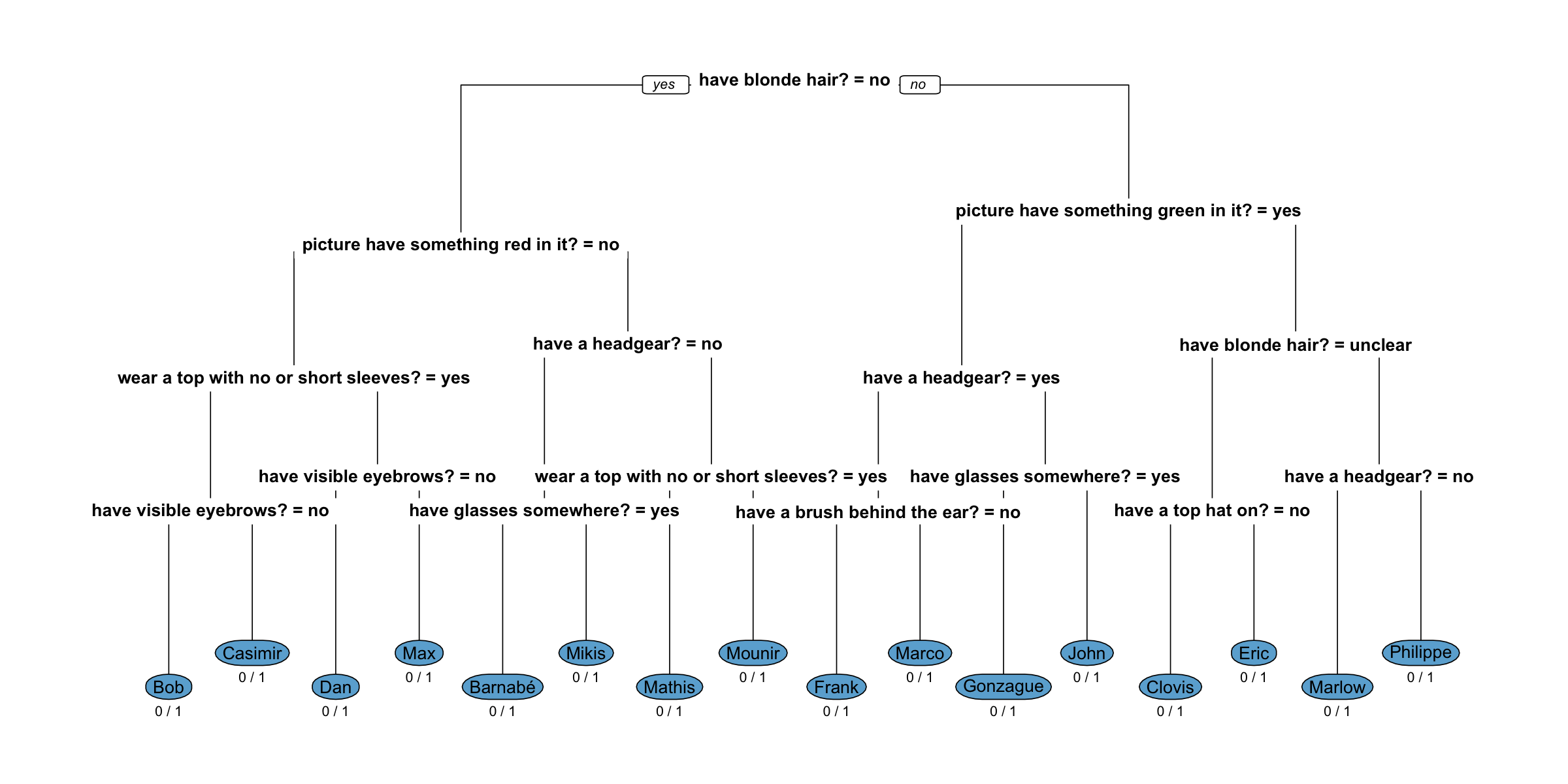
Figure 2: Decision tree to correctly identify your opponent with 4 questions.
We note that the misclassification rate at each terminal leaf is 0, i.e. if we follow the decision tree we are able to identify the correct person. Furthermore, the depth of the tree is only 4. Hence, even though there are 12 questions, the decision trees shows that we can use them in a clever sequence so that - no matter how the answer is - we correctly identify the person after 4 questions. Only 9 out of the 12 questions are used anywhere in the tree.
Discussion
Finding optimal sequences of question for identification has application beyond winning logic games. One example is fault tree diagnosis in reliability assessment, where entropy also plays a central role in the finding minimal cut set (Xiaozhong 1991). Troubleshooting complex technical devices, such as printers, in addition to a dianosis stage can also model the consequence of any repair actions (Langseth and Jensen 2003).
References
Appendix: Technical Details
This section discusses the algorithmic details of how classification trees are grown. For readers without interest in such technical detail this section can safely be skipped. More details can be found in for example Hastie, Tibshirani, and Friedman (2017), Sect 9.2.3.
The number of possible splits for a categorical node with \(M\) unordered categories is \(2^{M-1}-1\), i.e. for \(M=2\) features there is only one possible split, whereas \(K=3\) features have 3 possible splits. In our case, questions with \(M=2\) have answers yes and no and thus the split is ({yes}, {no}). When \(M=3\) we have answers yes, no and unclear and consequently the splits are: ({yes}, {no, unclear}), ({yes, unclear}, {no}), and ({yes,no},{unclear}). Note that most questions in the question catalogue have \(K=2\) answers:
persons %>% summarise(across(-Person, n_distinct))  %>%
  pivot_longer(cols=everything(), values_to = "M") %>%
  group_by(M) %>%
  summarise(no_questions=n())
## # A tibble: 2 × 2
## M no_questions
## <int> <int>
## 1 2 11
## 2 3 1Let the learning set be \(\mathcal{L}=\{ (\boldsymbol{x}_i, y_i), i=1,\ldots,n\}\), where \(\boldsymbol{x}_i=(x_{i1},\ldots,x_{ir})^\top\) denotes the answers to the \(r=12\) questions for each of the \(n=16\) persons on a game card. For a node \(m\) in tree \(T\) we use an impurity measure \(Q_m(T)\) to decide which split to use. Let \(R_m\) denote the set of all observations in the training data, whose feature vector \(\boldsymbol{x}_i\) fulfills all Boolean conditions posed by following the tree until node \(m\). In what follows we shall write \(\boldsymbol{x}_i\in R_m\) if an observation \((\boldsymbol{x}_i, y_i)\) from the learning data is in \(R_m\). Furthermore, let \(n_m=|R_m|\) denote the corresponding number of observations in \(R_m\) and let \[ \widehat{p}_{mk}=\frac{1}{n_m} \sum_{\boldsymbol{x}_i\in R_m} I(y_i=k) = \frac{n_{mk}}{n_m}, \quad k=1,\ldots,K \] be the proportion of category \(k\) observations at node \(m\). The cross-entropy impurity measure is defined as
\[ Q_m(T) = - \sum_{k=1}^K \widehat{p}_{mk} \cdot \log(\widehat{p}_{mk}), \] where we use the convention that \(0\cdot \log(0)=0\) if some of the probabilities \(\widehat{p}_{mk}\) are zero. As an example we show a plot of the cross-entropy function for \(K=2\) for varying values of \(p_{m1}=p\) and \(p_{m2}=1-p\):
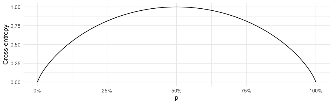
The largest value for the impurity \(Q_m(T)\) is obtained when all \(K\) categories are equally likely, i.e. when \(p_{mk}=1/K\), \(k=1,\ldots,K\). Furthermore, the smallest value \(Q_m(T)=0\) is obtained when one category, say \(k\), has \(p_{mk}=1\) and consequently \(p_{mk'}=0\) for all \(k' \neq k\).
For a node \(m\) and unordered categorical feature \(x_j\), \(j=1,\ldots,r\) we can now investigate the set of possible splits \(S_j\) of \(x_j\) by looking at the gain in impurity for each split \(s\in S_j\). A split \(s=(s_L, s_R)\) of \(x_j\) is characterised by a partition of the labels of \(x_j\) in two disjoint sets, \(s_L\) and \(s_R\). For example, if \(x_j\) has \(M=3\) levels (yes, no, unclear) one possible split could be \(s_L=\{\text{yes\}}\) and \(s_R=\{\text{no,unclear}\}\).
If we split \(m\) according to the rule \(s\in S_j\) we obtain two sub-nodes \(m_L\) and \(m_R\), where \(R_{m_L} = \{ \boldsymbol{x}_i \in R_m : x_{ij} \in s_L\}\) and \(R_{m_R} = \{ \boldsymbol{x}_i \in R_m : x_{ij} \in s_R\}\). The impurity of \(m\) in a tree \(T_s\) implementing the split \(s\), and thus having additional subnodes \(m_L\) and \(m_R\), is then calculated as \[ Q_m(T_s) = \frac{n_{m_L}}{n_m} Q_{m_L}(T_s) + \frac{n_{m_R}}{n_m} Q_{m_R}(T_s). \] Note that the probabilities to be used in the computation of the subnodes’ cross-entropy are, e.g., \(\widehat{p}_{m_L k} = n_{m_L k}/n_{m_L}\). We select the split, which minimizes the impurity. If we also let the feature \(j\) vary we thus select \[ (j,s)=\DeclareMathOperator*{\argmin}{arg\,min} \argmin_{j\in\{1,\ldots,r\},\> s\in S_j} Q_m(T_s). \] As a simple example for our data: assume that the current tree consists of just a root node \(m\), i.e. \(R_m\) consists of all \(n=16\) observations.
# Compute impurity of root
(Q_root <- cross_entropy(rep(1/16, 16)))
## [1] 2.772589# Determine if split on feature j
best_split <- function (j, Rm) {
# We know |S|=2^{M-1}-1 and define the split by the set consisting of
# just ONE level (if |S|=1 we know yes/no and would not need the other level.
# We can just pick one of them
S <- levels(persons[,j][[1]])
if (length(S) == 2) S <- S[2]
if (length(S) > 3) stop("M>3 currently not supported.")
S
# Try out all splits
Q_s <- sapply(S, function(s) {
R_mL <- Rm[Rm[,j][[1]] == s,]
R_mR <- Rm[Rm[,j][[1]] != s,]
n_m <- nrow(Rm)
n_mL <- table(R_mL$Person)
n_mR <- table(R_mR$Person)
p_mL <- n_mL / sum(n_mL)
p_mR <- n_mR / sum(n_mR)
Q_s <- sum(n_mL)/n_m * cross_entropy(p_mL) + sum(n_mR)/n_m * cross_entropy(p_mR)
return(Q_s)
})
tibble(name = names(Rm)[j], split=S[which.min(Q_s)], Q=min(Q_s))
}
# Columns of the data frame where the questions are located
question_col_idx <- seq_len(ncol(persons))[-1]
e <- map_df(question_col_idx, best_split, Rm=persons) %>% arrange(Q)
head(e)## # A tibble: 6 × 3
## name split Q
## <chr> <chr> <dbl>
## 1 have blonde hair? no 2.08
## 2 picture have something red in it? yes 2.09
## 3 have a headgear? yes 2.15
## 4 wear a top with no or short sleeves? yes 2.15
## 5 have visible eyebrows? yes 2.15
## 6 have blue eyes? yes 2.15If we are to build the tree only with one additional node we would thus use the Does the person have blonde hair? question and would put the no answers in one branch the yes and unclear answers on the other branch.
The same computations can be done with the
rpart::rpart() function. We set the control parameters s.t.
the tree can consist only of one split (maxdepth=1).
Furthermore, we lower the minimum number of observations one split can
produce in one branch from the default value of 20. Otherwise, with only
16 observations no split would be attempted.
tree_onesplit <- rpart(Person ~ ., data = persons, method="class",
               parms=list(split="information"),
               control=rpart.control(minsplit=1,  maxdepth=1))
rpart.plot(tree_onesplit, under=TRUE, extra=3, box.palette="Blues")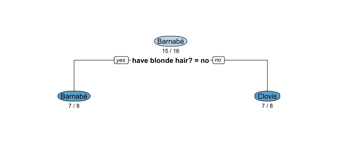
The graph of the decision tree in each node contains the most likely class. The number below the most likely class specifies the misclassification rate from this choice. As all classes are initially equally likely, choosing “Barnabé” at the root node (i.e. if it is not possible to ask further question) is just the first alphabetical choice - selecting any of the 15 other persons would have resulted in the same misclassification error. Similarly, choosing “Barnabé” among those with no blonde hair (somewhat confusingly this corresponds to the branch labelled “yes” of the logical condition: Does the person have blonde hair = no) is again just for alphabetical reasons. Equally probable classifications would have been Mounir, Dan, Barnabé, Casimir, Max, Bob, Mathis and Mikis. This is also reflected by the misclassification rate in that leaf node, which is 7/8.
Assume now that we picked the blonde hair question and are ready to add an additional sub-node to each of the two branches: Which question should we choose in each case?
R_L <- persons %>% filter(`have blonde hair?` == "no")
map_df(question_col_idx, best_split, Rm=R_L) %>% slice_min(order_by=Q)
## # A tibble: 1 × 3
## name split Q
## <chr> <chr> <dbl>
## 1 picture have something red in it? yes 1.39R_R <- persons %>% filter(`have blonde hair?` != "no")
map_df(question_col_idx, best_split, Rm=R_R) %>% slice_min(order_by=Q)## # A tibble: 1 × 3
## name split Q
## <chr> <chr> <dbl>
## 1 picture have something green in it? yes 1.39In other words, for the branch where
have blonde hair? == "no" we ask, whether the person’s
picture has something red in it, whereas we for those with blonde or
unclear hair color ask, if there is something green in the person’s
picture. Again, we can reproduce this directly using
rpart::rpart().
tree_twosplit <- rpart(Person ~ ., data = persons, method="class",
               parms=list(split="information"),
               control=rpart.control(minsplit=1, maxdepth=2))
As before, the selected person at each node is again a purely alphabetical choice, e.g. at the leftmost leaf node (Bob) equally probable choices would have been Dan, Casimir, Max and Bob. The above classification tree is of course still not perfect with misclassification rates of 3/4 at each leaf node. In the main section of the blog post we compute a more elaborate decision tree with a depth of 4 having zero misclassification rate at each leaf node.