Risky Risk Results
Abstract:
We determine the probabilities of winning battles in the dice-based board game Risk by counting and using Markov chains. The results show that if the battle is executed with 5 or more armies, the attacker has a slight advantage when both the attacker and defender start with the same number of armies.
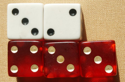
Image source: Wikipedia
 This work is licensed under a Creative Commons
Attribution-ShareAlike 4.0 International License. The R-markdown
source code of this blog is available under a GNU General Public
License (GPL v3) license from GitHub.
This work is licensed under a Creative Commons
Attribution-ShareAlike 4.0 International License. The R-markdown
source code of this blog is available under a GNU General Public
License (GPL v3) license from GitHub.
Introduction
While watching yet another episode of Numberphile, I was puzzled by a statement from Marcus du Sautoy about how people initially got the analysis of probabilities in the game of Risk wrong. Digging a little deeper, du Sautoy (2023) on pp. 306-307 refers to erroneous probability calculations made by Tan (1997), which were subsequently corrected by Osborne (2003) using counting techniques. What surprised me was that Tan (1997) could have easily spotted the error with a simple Monte Carlo simulation (see Appendix 1). This story about risky risk results for Risk has become a motivating example in my Probability 101 class on why Monte Carlo simulations are important.
In what follows, I shall focus on computing the necessary probabilities by counting. Several literature sources, including the aforementioned Tan (1997), Osborne (2003), as well as Pierce and Wooster (2015) and Hendel et al. (2015), calculate the probabilities. However, I was not able to find any publicly available programming code to verify their claims. Hence, the goal of this post is to provide literate programming style documented open-source R code to compute these probabilities.
Mathematical Description of a Single Battle
In the Game of Risk a single battle between \(a\) attacking armies and \(d\) defending armies is carried out as follows: Both the attacker and the defender roll one six-sided die for each of their armies inolved in the battle. The highest die of the attacker is then compared to the highest die of the defender. If the attacker’s die is higher, then the defender loses one army, otherwise the attacker loses one army. If both the attacker and the defender use more than one army, the next-highest dice are compared, and the process is repeated. The game imposes the restrictions \(a \in {1,2,3}\) and \(d \in {1,2}\) for a single battle.
Denote by \(Y_{1}, \ldots, Y_{a}\) independent random variables representing the outcomes of the \(a\) dice rolled by the attacker. Similarly, denote by \(Z_{1}, \ldots, Z_{d}\) independent random variables representing the outcomes of the defender’s \(d\) dice. Each of these \(a+d\) random variables follows a discrete uniform distribution, i.e. \(U(\{1,\ldots,6\})\). Furthermore, let \(Y_{(1)}\geq \cdots \geq Y_{(a)}\) and \(Z_{(1)}\geq \cdots \geq Z_{(d)}\) denote the ordered outcomes of the attacker’s and defender’s dice, respectively.
The result of the first comparison is that the defender loses an army, if \(Y_{(1)}>Z_{(1)}\); otherwise, the attacker loses an army. If a second comparison is to be made – that is, if \(\min(a,d)=2\) – then the defender loses an army if \(Y_{(2)}>Z_{(2)}\); otherwise the attacker loses an army. Hence, a random variable describing the number of armies the defender loses in an \(a\) vs. \(d\) battle is \[ D = \sum_{i=1}^{\min(a,d)} I(Y_{(i)}>Z_{(i)}), \] where \(I(\cdot)\) is an indicator function that equals 1 if its argument is true and 0 otherwise. The variable \(D\) has support on the integer values \(0,\ldots,\min(a,d)\). Similarly, the number of armies the attacker loses is \(A = \min(a,d) - D\). Example: In the splash picture of the abstract, the attacker rolled 4,3,3 (red dice) and the defender 3,2 (white dice). Since \(4>3\) and \(3>2\), the defender loses two armies in this specific battle.
Denote by \(p_{adk}\) the probability that a single battle between \(a\) attacking armies and \(d\) defending armies results in the defender losing \(k\) armies, \(k=0,\ldots,\min(a,d)\). This probability can be computed by dividing the number of favourable outcomes by the total number of possible outcomes:
\[\begin{align} p_{adk} = \frac{1}{6^{a+d}}\sum_{y_1=0}^6 \cdots \sum_{y_a=0}^6 \sum_{z_1=0}^6 \cdots \sum_{z_d=0}^6 I\left(\left\{\sum_{j=1}^{\min(a,d)} I(y_{(j)}>z_{(j)})\right\} = k\right) \end{align}\]
Although this formula may look involved, the \(6^{a+d}\) is just the number of possible outcomes when throwing \(a+d\) dice and the summation over the indicator function is just a way to count all favourable configurations in the Cartesian product sample space \(\{1,\ldots,6\}^{a+d}\). Since the maximum values for \(a\) and \(d\) in Risk are 3 and 2, respectively, the dimension of the product space will be no larger than \(6^5=`6^5`\), which is tractable.
Computation
We start the R code by defining that we look at outcomes of the dice D6, i.e. the sample space of one dice is \(\Omega = \{1,\ldots,6\}\).
# Sample space for one dice throw
Omega <- 1:6
We then write a function, which uses the expand_grid()
function repeatedly in order to generate the Cartesian product \(\Omega^\text{nDice}\) for \(\text{nDice}\in\mathbb{N}\) dice.
Furthermore, we add a column containing the probability for each element
in this sample space, i.e. the probability is \(1/|\Omega|^{\text{nDice}}=1/6^{\text{nDice}}\),
since the dice are assumed to be fair.
# Do expand_grid on the \Omega set sequentially a given number of nDice times.
# At the end we have nDice columns.
#
# @param nDice (integer) We compute \Omega_{dice}^{nDice}
# @param Omega (vector of integers) The faces on the dice.
#
# @return Tibble with nDice columns containing all |\Omega_{dice}|^{nDice} possible outcomes and a column stating the probability of each element in this sample space, i.e. 1/|\Omega_{dice}^{nDice}|.

sample_space <- function(nDice, Omega=1:6) {
 expand_grid(!!!replicate(nDice, Omega, simplify = FALSE)) %>%
   setNames(str_c("D", 1L:nDice)) %>%
    mutate(prob = 1/(length(Omega)^nDice))
}
Instead of calculating a matrix containing all possible outcomes of the \(a+d\) dice, as in the sum-formula above, and then handling the sorting, we divide the problem into two tasks:
- Calculate all possible outcomes and their probabilities when sorting the outcome of the attacker’s \(a\) dices
- Calculate all possible outcomes and their probabilities when sorting the outcome of the attacker’s \(d\) dices
Since the dice throws of the attacker and defender are independent, we can then compute the required joint distribution by multiplying the two marginal distributions found in 1. and 2.
As a consequence we write a function that returns all possible outcomes of \(Y_{(1)} \leq \ldots \leq Y_{(\text{nCompare})}\) obtained after ordering the outcome of dice, i.e. \(Y_{(1)} \leq \ldots \leq Y_{(\text{nDice})}\) with \(\text{nCompare} \leq \text{nDice}\). To be compatible with the game of risk \(\text{nCompare}\in\{1,2\}\). We compute the associated probabilities by adding up the underlying entries of the Cartesian sample space.
combos_sorted <- function(nDice=3, nCompare=min(2,nDice), base_name = "y") {
  # Generate all outcomes and make a label
  # which identifies which of the sorted bins the outcome belongs to
  combos <- sample_space(nDice=nDice) %>%
    rowwise() %>%
    mutate(combo_sorted = str_c(sort(c_across(all_of(paste0("D", 1:nDice))), decreasing=TRUE), collapse=""),
           combo_label = str_sub(combo_sorted, 1, nCompare))

  # Count accoring
  combos_summed <- combos %>% group_by(combo_label) %>%
    summarise(n=n(), prob=sum(prob)) %>%
    arrange(desc(combo_label)) %>%
    # We use the notation by Osborn (2009) and denote the columns y^{(1)} \geq y^{(2)} \geq y^{(3)}
    separate_wider_position(cols = combo_label, widths = set_names(rep(1, nCompare), nm= str_c(base_name, "_{(", 1:nCompare,")}")))

  # Done
  return(combos_summed)
}
As an example:
combos_sorted(nDice=3, nCompare=2)## # A tibble: 21 × 4
## `y_{(1)}` `y_{(2)}` n prob
## <chr> <chr> <int> <dbl>
## 1 6 6 16 0.0741
## 2 6 5 27 0.125
## 3 6 4 21 0.0972
## 4 6 3 15 0.0694
## 5 6 2 9 0.0417
## # ℹ 16 more rowsThis can then be combined to obtain the joint distribution of the sorted dice to be compared.
joint_combos_sorted <- function(a, d) {
  # Sort the throws of the attacker and defender
  Y <- combos_sorted(nDice=a, base_name="y")
  Z <- combos_sorted(nDice=d, base_name="z")

  # Make a tibble with all combinations of the a vs. d armies fight
  joint <- Y %>% cross_join(Z) %>%
    mutate(prob = prob.x * prob.y,
           n = n.x * n.y) %>%
    select(-n.x, -n.y, -prob.x, -prob.y)

  #Done
  return(joint)
}
Which for a single \(a=3\) vs. \(d=2\) battle would look like:
head(joint_combos_sorted(a=3, d=2), n=3)## # A tibble: 3 × 6
## `y_{(1)}` `y_{(2)}` `z_{(1)}` `z_{(2)}` prob n
## <chr> <chr> <chr> <chr> <dbl> <int>
## 1 6 6 6 6 0.00206 16
## 2 6 6 6 5 0.00412 32
## 3 6 6 6 4 0.00412 32We can now compute \(p_{adk}\) by comparing \(Y_{(i)}>Z_{(i)}\) for all relevant \(i=1,\ldots,\min(a,d)\) and summing all outcomes where the defender loses \(k\) armies:
########################################################################
# Distribution over the number of armies that defender is losing,
# when attacker is using A armies and defender is using D armies.
#
# @param A Number of armies (=dice) the attacker sends into the battle
# @param D Number of armies (=dice) the defender sends into the fight
#
# @return A tibble containing all possible outcomes of the battle in terms
#         of losses for attacker and defender.
########################################################################
p_lose_ad <- function(a=3, d=2) {
  # All joint combinations of attacker and defender
  joint <- joint_combos_sorted(a=a, d=d)

  # Number of dice to compare
  nCompare <- pmin(a, d)

  # I find this loop version easier to understand
  # than a corresponding tidyverse version
  for (k in seq_len(nCompare)) {
    joint[, str_c("lose_D_pos", k)] <- (joint[,str_c("y_{(",k,")}")] > joint[,str_c("z_{(",k,")}")])
  }

  # Total sum of armies lost by defender and attacker, respectively
  joint <- joint %>%
    mutate(lose_D = rowSums(select(., matches("^lose_D_pos[0-9]+"))),
           lose_A = nCompare - lose_D)  %>%
    select(starts_with("y"), starts_with("z"), prob, lose_A, lose_D)

  # Add up probabilities for all combos yielding a specific
  # lose_A, lose_D combo
  res <- joint %>% group_by(lose_A, lose_D) %>%
    summarise(prob = sum(prob), .groups="drop") %>%
    arrange(lose_D)

  # Done
  return(res)
}
To test the function, we compute \((p_{320},p_{321},p_{322})\), which Osborne (2003) found to be \((2275, 2611, 2890)/7776=(0.293,0.336,0.372)\):
# 3 vs. 2 battle
p_lose_ad(a=3, d=2)
## # A tibble: 3 × 3
## lose_A lose_D prob
## <dbl> <dbl> <dbl>
## 1 2 0 0.293
## 2 1 1 0.336
## 3 0 2 0.372# Check that p_lose_ad is correct for p_{32k}, k=0,1,2
all.equal(p_lose_ad(a=3, d=2) %>% pull(prob), c(2275, 2611, 2890)/7776)## [1] TRUEAn alternative verification is to use the Troll dice roller and probability calculator by Torben Æ. Mogensen using the following syntax:
a:=3d6;b:=2d6;
count {(max a)>(max b),(min largest 2 a)>(min b)}
Troll computes the probability distribution as:
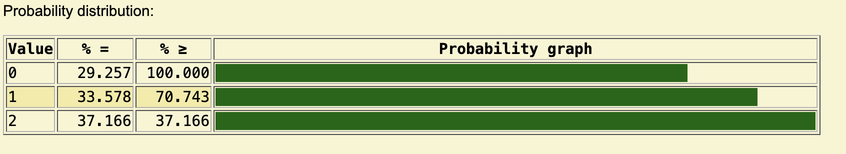
Figure 1: Results for the 3 vs. 2 risk roll in Troll.
Note that for the \(p_{32k}, k=0,1,2\) setup, Tan (1997) instead obtained \((0.237, 0.504, 0.259)\), which differs substantially from the correct result. See Appendix 2 for a discussion of his calculations.
The complete table of probabilities for all possible single battle attacker vs. defender configurations can now be computed as follows:
state_change <- expand_grid(a=1:3, d=1:2) %>% rowwise() %>%
  mutate(prob = list(p_lose_ad(a=a, d=d))) %>%
  unnest(prob)
## Warning: `...` must be empty in `format.tbl()`
## Caused by error in `format_tbl()`:
## ! `...` must be empty.
## ✖ Problematic argument:
## • row.names = FALSE## # A tibble: 14 × 4
## a d k prob
## <int> <int> <dbl> <dbl>
## 1 1 1 0 0.583
## 2 1 1 1 0.417
## 3 1 2 0 0.745
## 4 1 2 1 0.255
## 5 2 1 0 0.421
## 6 2 1 1 0.579
## 7 2 2 0 0.448
## 8 2 2 1 0.324
## 9 2 2 2 0.228
## 10 3 1 0 0.340
## 11 3 1 1 0.660
## 12 3 2 0 0.293
## 13 3 2 1 0.336
## 14 3 2 2 0.372Voila! The values align with those in Table 2 of Osborne (2003).
Repeated Battles using Markov Chains
Once the probabilities for army losses of a single battle have been computed, the natural follow-up question is: what happens if the attacker decides to continue the attack? Assume that the attacker continues to battle with as many armies as possible until either the attacker has no armies left to attack with or the defender is destroyed, i.e. has no armies left. What is the probability of an attacker with \(A\geq 1\) armies winning such a repeated attack against a defender with \(D\geq 1\) armies?
As stated in Osborne (2003), this is elegantly solved using Markov chains. Denote by \((A,D)\) the current state of the chain with \(A\) attacking armies and \(D\) defending armies. Assuming that both attacker and defender use as many dice possible, i.e. \(a=\min(3,A)\) and \(d=\min(2,D)\), the next battle would be a 3 vs. 2 battle if \(A\geq 3\) and \(D\geq 2\). Hence, the attacker can lose \(0,1,2\) armies, while the defender can lose \(0,1,2\) armies. No matter the outcome, 2 armies will be lost in the battle. Therefore, the new state is: \[ (A,D) \longrightarrow \left\{ \begin{array}{cl} (A-2, D) & \text{with probability } \pi_{320} \\ (A-1, D-1) & \text{with probability } \pi_{321} \\ (A, D-2) & \text{with probability } \pi_{322} \end{array} \right. \] If \(A\) and/or \(D\) are smaller than 3 and 2, the transitions and its probabilities changes accordingly. Note that once either \(A\) or \(D\) is zero, the state is absorbing, meaning it is no longer possible to continue the battle, and the state will remain the same. If after updating \(A=0\), the attacker has lost the fight1. However, if \(D = 0\), the defender loses, and the attacker conquers the country.
# Armies at the start of the battle
A <- 10
D <- 10
size_state_space <- (A+1)*(D+1)
Suppose we start with \(A=10\)
attacking armies and \(D=10\) defending
armies. The corresponding state space of the Markov chain is \(\{(A, D), A\in\{0,\ldots,10\}, D\in
\{0,\ldots,10\}\}\). Mapping this to a vector means creating a
vector of length \(11 \times 11=121\).
Hence, the transition matrix \(P\) will
be \((121\times121)\) matrix. We also
note that the transition matrix will be sparse, i.e. only a couple of
its cells will be non-zero. As a consequence, we can use appropriate
storage techniques from the Matrix
package to make efficient use of sparseness for example when doing
matrix multiplications. The function
transition_matrix(A, D) handles all these steps and sets up
the transition matrix P.
The vector representing the situation with \(10\) attacking armies and 10 defending armies would be \(\mathbf{x}_0=(0,\ldots,0, 1)^\top\). The development in probabilities over the state space after a single battle can then be represented as \(\mathbf{x}_1 = \mathbf{x}_0^\top\mathbf{P}\). Starting in state \((10,10)\) we can thus go to either \((8,10)\), \((9,9)\) or \((10,8)\) and we recognize \(p_{320}\), \(p_{321}\) and \(p_{322}\) as the transition probabilities.
x0 <- states$state == sprintf("%2d-%2d",A,D) # "10-10"
x1 <- t(x0) %*% P
x1[, as.logical(x1>0)]
## 08-10 09-09 10-08
## 0.2925669 0.3357767 0.3716564Subsequent battles are implemented as \(\mathbf{x}_{i+1} = \mathbf{x}_{i}^\top \mathbf{P}\). For each single battle, the total number of armies will decrease by at least 1 army (and most likely 2). Starting with \(A+D\) armies means that after \(A+D\) battles we are guaranteed to have reached an absorbing state, i.e. a state which is characterized by either its first or second component being zero, i.e. the absorbing states are \((0,D),(0,D-1),\ldots,(0,1),(1,0),\ldots,(A-1,0),(A,0)\). Note that there are exactly \(A+D\) absorving states, because the outcome \((0,0)\) can not occur. Considering \[ \mathbf{x}_{A+D} = \mathbf{x}_{0}^\top \mathbf{P}^{A+D} = \mathbf{x}_{0}^\top \underbrace{\mathbf{P} \cdots \mathbf{P}}_{\text{$A+D$ times}} \] we compute
x_AD <- t(x0) %*% matpow(P, A+D)
x_AD[, as.logical(x_AD>0)]
## 00-01 00-02 00-03 00-04 00-05 00-06 00-07 00-08 00-09 00-10 01-00 02-00 03-00 04-00 05-00 06-00 07-00 08-00 09-00 10-00
## 0.042 0.081 0.072 0.070 0.056 0.047 0.031 0.021 0.009 0.003 0.030 0.059 0.092 0.096 0.087 0.077 0.059 0.039 0.021 0.007Summing up all probabilities where the defender has zero armies gives us the probability that the attacker wins the battle, i.e.
sum(x_AD[,str_detect(colnames(x_AD), "-00")])## [1] 0.5675929This probability matches the value 0.568 reported in Table 3 of Osborne (2003). Note that the above \((A+D)\)-move computations takes a more direct route for the computation than Osborne (2003) – see Appendix 3. By calculating \(\mathbf{P}^{A+D}\) once, we can change the initial state vector \(\mathbf{x}_0\) to compute the probability of the attacker winning for each of the \(A \times D\) possible initial values. The values match those in Table 3 of Osborne (2003).
| A | 1 | 2 | 3 | 4 | 5 | 6 | 7 | 8 | 9 | 10 |
|---|---|---|---|---|---|---|---|---|---|---|
| 1 | 0.417 | 0.106 | 0.027 | 0.007 | 0.002 | 0.000 | 0.000 | 0.000 | 0.000 | 0.000 |
| 2 | 0.754 | 0.363 | 0.206 | 0.091 | 0.049 | 0.021 | 0.011 | 0.005 | 0.003 | 0.001 |
| 3 | 0.916 | 0.656 | 0.470 | 0.315 | 0.206 | 0.134 | 0.084 | 0.054 | 0.033 | 0.021 |
| 4 | 0.972 | 0.785 | 0.642 | 0.477 | 0.359 | 0.253 | 0.181 | 0.123 | 0.086 | 0.057 |
| 5 | 0.990 | 0.890 | 0.769 | 0.638 | 0.506 | 0.397 | 0.297 | 0.224 | 0.162 | 0.118 |
| 6 | 0.997 | 0.934 | 0.857 | 0.745 | 0.638 | 0.521 | 0.423 | 0.329 | 0.258 | 0.193 |
| 7 | 0.999 | 0.967 | 0.910 | 0.834 | 0.736 | 0.640 | 0.536 | 0.446 | 0.357 | 0.287 |
| 8 | 1.000 | 0.980 | 0.947 | 0.888 | 0.818 | 0.730 | 0.643 | 0.547 | 0.464 | 0.380 |
| 9 | 1.000 | 0.990 | 0.967 | 0.930 | 0.873 | 0.808 | 0.726 | 0.646 | 0.558 | 0.480 |
| 10 | 1.000 | 0.994 | 0.981 | 0.954 | 0.916 | 0.861 | 0.800 | 0.724 | 0.650 | 0.568 |
All cells with a probability greater than 0.5 are colored green in the table. We observe that from 5 and beyond the attacker has a slight advantage when \(A=D\).
Below, the situation for \(A,D\) up to 50 is illustrated a little differently: for any given value of \(D\), the image shows in green all values of \(A\), where the probability for the attacker to win is above 50%.
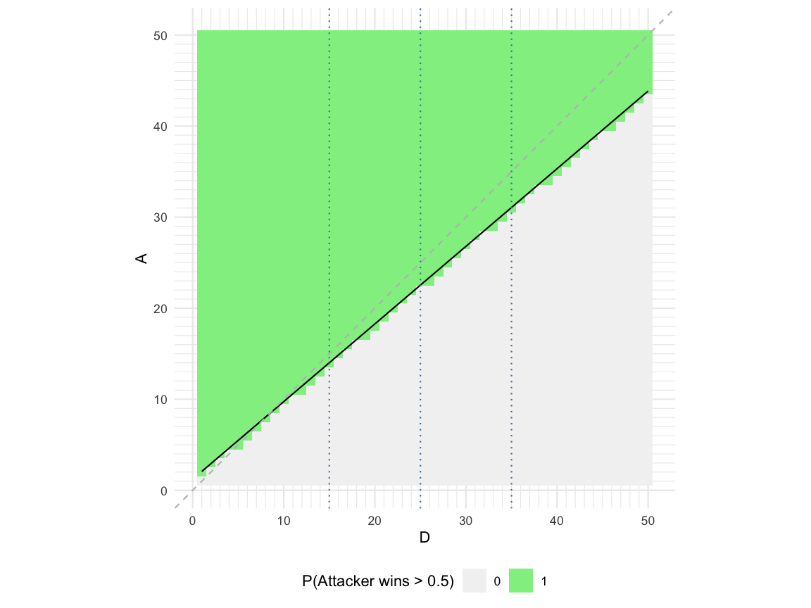
Looking at the smallest \(A\) with a win probability of more than 50% for a given \(D\), we see that this line is below the \(A=D\) line. This shows that the attacker has a slight advantage. Furthermore, the smallest such \(A\) can be found approximately as \(A_{\min} \approx 1.2204 + 0.8525\cdot D\).
Another way to illustrate the findings is by slicing the table of probabilities for a given value of \(D\). In the previous plot, slices for \(D=15,25,35\) are shown. Given the value of \(D\), the corresponding probability for the attacker to win as a function of the number of attacking armies is shown below:
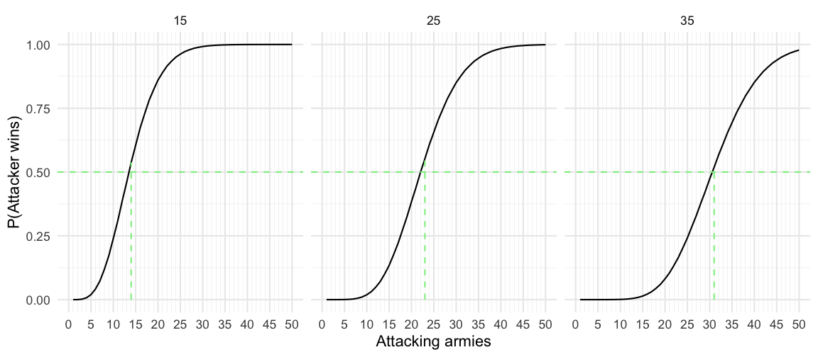
The vertical line in each plot shows the smallest number of attacking armies, s.t. the probability of the attacker winning is greater than 50%. The values are 14,23,31, respectively.
To get an impression of how many armies are lost as part of an \(A\) vs. \(D\) battle, let \(\Delta\) denote a random variable describing the number of armies the attacker has left at the end of the battle minus the number of armies the defender has left at the end. Note that since the battle ended, either the attacker or the defender must have zero armies left. The support of \(\Delta\) is \(\{-D,\ldots,-1,1,\ldots,A\}\); below is shown the corresponding probability mass function (PMF) of \(\Delta\) for the 50 vs. 50 battle.
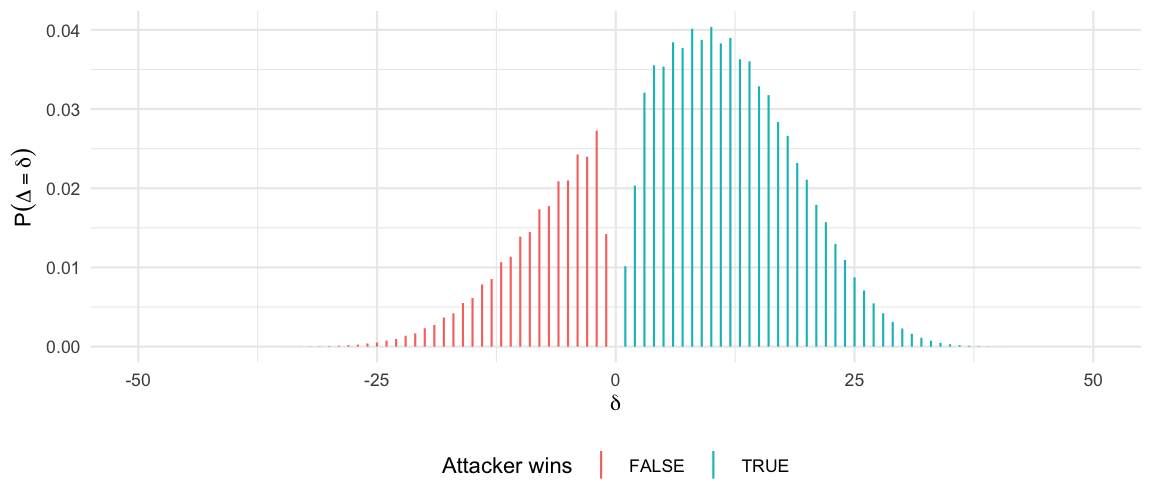
Note that if \(\Delta>0\), then the attacker wins. Hence, for better visualization, the plot of this sawtooth shaped PMF is colored using the two outcomes of the battle. The overall probability for the attacker to win is 73.6%, which can be found as the sum of the cyan bars. If focus is restricted to the number of armies the attacker loses during the attack, one could instead consider \(L:=\max(0,\Delta)\), which corresponds to stacking all red bars of the PMF in the value 0, while keeping the cyan part. The expected number of armies the attacker looses in a battle won is then \(A-\operatorname{E}(L|L>0)\), which for the given 50 vs. 50 battle means that the attacker is expected to lose 37.8 armies when winning.
Discussion
Counting is a powerful technique in combinatorics and dice-based probabilities. The counting can be implemented on a computer by representing the full sample space using tables or arrays. The risk of making mistakes when counting in such structures is often lower than in more involved probability calculations, e.g. order statistics or conditional distributions. However, in many combinatorical problems the state space quickly exceeds manageable sizes. Monte Carlo simulation offers a quick alternative for verifying probability calculations, and is effective even in untractably large state spaces.
TLDR: For situations where \(A \geq 5\), attack if \(A \geq 1.2204 + 0.8525\cdot D\).
Appendix 1: Monte Carlo Simulation
Just for completeness: Below is a simulation function for determining the \(p_{adk}\) probabilities by Monte Carlo simulation. It requires little thinking, is fast and accurate enough to spot the errors in the Tan (1997) paper:
# Simulate a single a vs. d army battle
single_battle <- function(a = 3, d = 2) {
  # Sort the dice
  y_sorted <- sort(sample(Omega, size = a, replace = TRUE), dec = TRUE)
  z_sorted <- sort(sample(Omega, size = d, replace = TRUE), dec = TRUE)

  # Number of comparisons
  nCompares <- min(a, d)

  # For each position to compare, see if defender looses an army.
  lose_D <- (y_sorted[1:nCompares] > z_sorted[1:nCompares])

  return(sum(lose_D))
}

# Calc p_{32k}, k=0,1,2
prop.table(table(replicate(1e5, single_battle(a=3, d=2))))
##
## 0 1 2
## 0.29136 0.33852 0.37012Appendix 2
Tan (1997) calculated for example \[\begin{align*} \pi_{322} &= P(Y_{(1)}>Z_{(1)} \cap Y_{(2)}>Z_{(2)}) \\ &= P(Y_{(1)}>Z_{(1)}) P(Y_{(2)}>Z_{(2)}) \\ &= \cdots, \end{align*}\] but the 2nd step is wrong, because it assumes independence of the events \(Y_{(1)}>Z_{(1)}\) and \(Y_{(2)}>Z_{(2)}\). This is not the case, as seen from the following R output:
# Joint distribution of the two events
f_Y12Z12 <- joint_combos_sorted(a=3, d=2) %>%
  mutate(`y_{(1)}>z_{(1)}`=`y_{(1)}`> `z_{(1)}`,
         `y_{(2)}>z_{(2)}`=`y_{(2)}`> `z_{(2)}`) %>%
  group_by(`y_{(1)}>z_{(1)}`,`y_{(2)}>z_{(2)}`) %>%
  summarise(prob=sum(prob), .groups = "keep")

# Marginal distribution of each event
f_Y1Z1 <- f_Y12Z12 %>% group_by(`y_{(1)}>z_{(1)}`) %>% summarise(prob=sum(prob))
f_Y2Z2 <- f_Y12Z12 %>% group_by(`y_{(2)}>z_{(2)}`) %>% summarise(prob=sum(prob))

# Joint prob when **assuming independence**
f_Y12Z12_indep <- cross_join(f_Y1Z1, f_Y2Z2) %>%
  mutate(prob_indep = prob.x * prob.y) %>%
  select(-prob.x,-prob.y)

# Compare to the true joint distribution: this is definitely not the same!
inner_join(f_Y12Z12, f_Y12Z12_indep, by=c("y_{(1)}>z_{(1)}", "y_{(2)}>z_{(2)}"))
## # A tibble: 4 × 4
## # Groups: y_{(1)}>z_{(1)}, y_{(2)}>z_{(2)} [4]
## `y_{(1)}>z_{(1)}` `y_{(2)}>z_{(2)}` prob prob_indep
## <lgl> <lgl> <dbl> <dbl>
## 1 FALSE FALSE 0.293 0.207
## 2 FALSE TRUE 0.236 0.321
## 3 TRUE FALSE 0.0999 0.185
## 4 TRUE TRUE 0.372 0.286From the above output we notice that the correct joint distribution2 of the two events cannot be computed by simply multiplying the marginals. Hence, the two events are not independent.
The reason is that using order statistics induces dependencies. For example \(P(Z_{(1)}=z_1, Z_{(2)}=z_2) \neq P(Z_{(1)}=z_1) P(Z_{(2)}=z_2)\). Although the dice \(Z_1\) and \(Z_2\) are independent, the corresponding variables of the order statistics are dependent: knowing something about the higher of the two dice gives you information about the lower of the two. For example if you know that \(Z_{(1)}=1\), then you know for sure that \(Z_{(2)}=1\). This dependence extends to comparisons with the attacker’s dice.
Appendix 3
Osborne (2003) partitions the state space into transient and absorbing states and forms the transition matrix as a \(2\times 2\) block matrix between the two types, i.e. its canonical form (Grinstead and Snell 1997, Sect. 11.2) \[ \mathbf{P} = \begin{bmatrix} \mathbf{Q} & \mathbf{R} \\ \mathbf{0} & \mathbf{I} \end{bmatrix}, \] where \(\mathbf{Q}\) is the \((AD\times AD)\) transition matrix between transient states and \(\mathbf{R}\) is the \(AD\times (A+D)\) transition matrix between a transient state and an absorbing state. Finally, \(\mathbf{0}\) is the \((A+D)\times AD\) matrix of zeros, and \(\mathbf{I}\) is the \((A+D)\times(A+D)\) identity matrix. Altogether, \(\mathbf{P}\) has dimension \((AD+(A+D)) \times (AD+(A+D))\), which corresponds to the \((A+1)\times (D+1)\) dimension in the previous treatment, but explicitly disregards the (unreachable) state \((0,0)\).
Consider the probability that the Markov Chain \(\mathbf{X}\) at some point in time – without loss of generality we can assume this to be time 0 – is in state \(\mathbf{i}=(a,d)\), \(a,d\geq 1\) and then eventually moves on to the absorbing state \(\mathbf{j}\) in \(n\) steps, i.e. \[ \begin{align*} f_{\mathbf{ij}}^{(n)} &= P( \mathbf{X}_{n}= \mathbf{j} | \mathbf{X}_0=\mathbf{i} ) = \sum_{\mathbf{x}_{n-1}} \cdots \sum_{\mathbf{x}_1} P( \mathbf{X}_{n}= \mathbf{j}, \mathbf{X}_{n-1}= \mathbf{x}_{n-1},\ldots, \mathbf{X}_{1}= \mathbf{x}_{1}| \mathbf{X}_0=\mathbf{i} ) \\ &= \sum_{\mathbf{x}_{n-1}} \cdots \sum_{\mathbf{x}_1} P( \mathbf{X}_{n}= \mathbf{j}| \mathbf{X}_{n-1}= \mathbf{x}_{n-1})\cdots P(\mathbf{X}_{1}= \mathbf{x}_{1}| \mathbf{X}_0=\mathbf{i}) \end{align*} \] Let \(\mathbf{F}^{(n)}\) be the \(AD\times (A+D)\) matrix of all \(f_{\mathbf{ij}}^{(n)}\)’s. Since the first \(n-1\) moves have to be between transient states and the last move has to be a move between a transient state and an absorving state, we have \(\mathbf{F}^{(n)}=\mathbf{Q}^{n-1} \mathbf{R}\) when we define \(\mathbf{Q}^{0}=\mathbf{I}\). Summing over all possible sequence lengths \(n\) gives us the probability to eventually go from \(\mathbf{i}\) to \(\mathbf{j}\), i.e. \[ \mathbf{F} = \sum_{n=1}^\infty \mathbf{F}^{(n)} = \sum_{n=1}^\infty \mathbf{Q}^{n-1} \mathbf{R} = \left(\sum_{n=1}^\infty \mathbf{Q}^{n-1} \right) \mathbf{R} = (\mathbf{I}-\mathbf{Q})^{-1} \mathbf{R}, \] where the last equality follows from properties of the fundamental matrix of the absorbing Markov chain (Grinstead and Snell 1997, Thm. 11.4). The statement of the above equation corresponds to Theorem 11.6. in Grinstead and Snell (1997).
The probability that the attacker wins from a given initial condition \(\mathbf{i}\) can then be found by summing all entries of the \(\mathbf{i}\)’th row of \(\mathbf{F}\) corresponding to states where the defender has zero armies (and hence lost). One advantage of using the canonical form to compute the attacker’s win probabilities is that it is much faster to compute once \(A\) and \(D\) are big.
Literature
Since the rules of Risk only allow attacking with one army less than hosted in the country the attack originates from, the attacker would still have one army left once \(A=0\). Thus, the country is not yet lost but could be vulnerable to subsequent attacks in future rounds.↩︎
Obtained by counting using the involved sum-sum-indicator formula from above.↩︎