Dynamic Programming for Super Six

Abstract:

We use dynamic programming to find the optimal strategy for playing Super Six when there are 2 players. To test the cross-language capabilities of Rmarkdown we solve the task by embedding our Python implementation of the value iteration algorithm using the reticulate R-package.

This work is licensed under a Creative Commons Attribution-ShareAlike 4.0 International License. The R-markdown source code of this blog is available under a GNU General Public License (GPL v3) license from GitHub.

Introduction

The present post finds the optimal game strategy for playing the dice game of Super Six with two players by using dynamic programming to solve the corresponding Markov Decision Process (MDP). We use the reticulate R package to run our Python implementation of the value iteration algorithm within the Rmarkdown document.

For more details about Super Six, see the previous Blog post How to Win a Game (or More) of Super Six. Appendix 1 of the post discussed optimal strategies. The present post is a natural successor of this post, because it shows the details of calculating optimal strategies for two player games by value iteration Sutton and Barto (2020). This provides a clearer way to get to the strategy than, e.g., Jehn (2021) or the C++ program by Nuno Hulthberg.

Notation

In mathematical notation the current state \(s\) corresponds to the \(i/j/k\) situation, with \(0\leq i\leq 5\), \(j\geq 0\) and \(k\geq 0\).

In order to distinguish between the first turn of a player in a round (where the dice has to be thrown) and the subsequent turns, where the player can decide whether to throw the dice or stop, we add a fourth component \(l\in \{0,1\}\) to the state, which is a binary indicator whether the move is a forced moved (1) or not (0). The action space for a state \(i/j/k/l\) with \(l=1\) is \(\mathcal{A}(s) = \{\texttt{throw}\}\), whereas for \(l=0\) it is \(\mathcal{A}(s) = \{\texttt{throw},\texttt{stop}\}\).

If \(j=0\) while \(k>0\) then Player 1 won. If \(k=0\) while \(i>0\) then Player 2 won. In order to handle this episodic task (Sutton and Barto 2020) we introduce an terminal state, which provides no additional future reward.

State Transition

The state transition probabilities of the Markov decision process are given as follows. For each throw of the dice from an \(i/j/k/l\) state there are three cases to consider when throwing the dice:

1. you roll a six (probability \(\frac{1}{6}\)) and move to the \(i/(j-1)/k/0\) state
2. (if \(0\leq i< 5\)) you hit a free spot (probability \(\frac{5-i}{6}\)) and move to the \((i+1)/j/k/0\) state
3. (if \(0<i\leq 5\)) you hit an already occupied spot (probability \(\frac{i}{6}\)) and it is your opponents turn to play from an \((i-1)/k/(j+1)/1\) position

If you decide to stop throwing (only possible if \(l=0\)) then it is the opponent’s turn to play from an \(i/k/j/1\) position.

As part of the calculations one needs to know what happens if Player 1 looses their turn (i.e. either by hitting an occupied spot or by voluntarily deciding to stop) This depends on the strategy played by Player 2. For simplicity we will assume that Player 2 plays the same optimal strategy as Player 1. This also means that rewards in this situation are just minus the rewards obtained from the corresponding position.

Reward

Eventually, the game will finish. Let \(R(s,a,s')\) be the reward function, where action \(a\) moves the decision maker from state \(s\) to \(s'\). In our problem, the reward will only depend on \(s'\). We have \[ R(s'=(i,j,k,l)) = \left\{ \begin{array}{cl} 1 & \text{if $j=0$ and $k>0$} \\ -1 & \text{if $k=0$ and $j>0$} \\ 0 & \text{otherwise} \end{array} \right. \]

Side note: Since linear transformations of the reward function leave the optimal strategy unchanged (Sect. 17.1.3, Russell and Norvig 2020), it is equally possible to work with rewards \(R^*(s'=(i,j,k,l)) = \frac{1}{2}R(s'=(i,j,k,l)) + \frac{1}{2}\). This would imply values 1 for winning and 0 for loosing and translates directly the expected reward computations into computing expected probabilities for winning, which is what Jehn (2021) computed.

Bellman equations

The expected utility obtained from following stragy \(\pi\) is defined as \[ U^{\pi}(s) = E\left[ \sum_{t=0}^\infty R(S_t, \pi(S_t), S_{t+1})\right] \] The terminal state with future reward 0 ensures that \(U^\pi(s)<\infty\). No discounting of the rewards is thus used in our approach. Our aim is now to find a strategy \(\pi^*(s)\), which optimizes this expected utility, i.e. \[ \pi_s^* = \operatorname{argmax}_{\pi} U^{\pi}(s) \] For state \(s\) we thus choose the action that maximizes the reward for the next step plus the expected utility of the subsequent states: \[ \pi^*(s) = \operatorname{argmax}_{a\in \mathcal{A}(s)} \sum_{s'}P(s'| s,a) \left[ R(s,a,s') + \max_{a'} U(s') \right] \]

This expressions for a state \(s\) is also called the Bellman equation:

\[\begin{align*} U(s) &=\max_{a\in \mathcal{A}(s)} \sum_{s'}P(s'| s,a) \left[ R(s,a,s') + U(s') \right] \end{align*}\]

Hence, for a state \(i/j/k/0\) the action “continue” leads to to the following expansion of the sum term in the above equation:

\[ \begin{align*} & \underbrace{\frac{1}{6} [R(i/j-1/k/0) + U(i/j-1/k/0)]}_{\text{stick into hole}} \\ &+ \underbrace{\frac{5-i}{6} [R(i+1/j-1/k/0) + U(i+1/j-1/k/0)]}_{\text{put stick into lid}}\\ &- \underbrace{\frac{i}{6} [R(i-1/k/j+1/1) + U(i-1/k/j+1/1)]}_{\text{take stick from lid}} \end{align*} \] and the action to stop has value \(R(i-1/k/j+1/1) + U(i-1/k/j+1/1)\).

Value Iteration

We use value iteration (Sect. 17.2.1, Russell and Norvig 2020), (Sect 4.4, Sutton and Barto 2020) to solve the MDP. Let \(U(s)\) and \(U'\) be collections, which contain the value function for each \(s\) in the state space. We initialize \(U(s)=U'(s)=0\) for all states and proceed by the following algorithm:

Algorithm 1: Value iteration

repeat

1. \(U \gets U'; \delta \gets 0\)
2. For all states \(s\) do
   1. \(U'(s) \gets \max_{a\in \mathcal{A}(s)} \sum_{s'}P(s'| s,a) \left[ R(s,a,s') + U(s') \right]\)
   2. if \(|U(s')-U(s)| > \delta\) then \(\delta \gets |U(s')-U(s)|\)

until \(\delta \leq \epsilon\);

The optimal action for state \(s\) is thus the action maximing the sum term in Step 2a, i.e. \(\pi(s) = \operatorname{argmax}_{a\in \mathcal{A}(s)} \sum_{s'}P(s'| s,a) \left[ R(s,a,s') + \max_{a'} U(s') \right]\). Either one computes this at the end of the algorithm or one adds this book-keeping step as part of step 2a in the value iteration algorithm. Technically, \(\pi\approx \pi^*\), i.e. we only obtain an estimate of the optimal strategy, because of the iterative nature of the algorithm. However, one can show that with sufficient iterations we converge towards \(\pi^*\).

Results

Applying the value iteration Python code for \(n=7\) (see code in the Appendix) gives the optimal strategy. Furthermore, we also obtain the probabilities to win from each state. We show the result for all states with at least 3 sticks in the lid. With less than 3 sticks the decision is always to continue throwing.

In the output, the column strategy shows whether to continue throwing the dice (TRUE) or not (FALSE); the column value shows the expected value \(U(s)\) and prob shows the expected probability to win the game given that the opponent also follows the same optimal strategy. Note that for states with \(l=1\), no choice is possible, i.e. one has to continue no matter what. For these states the strategy column is always TRUE.

##    i j k l       value strategy      prob
## 1  5 1 1 1 -0.09741652     TRUE 0.4512917
## 2  5 1 1 0  0.09741652    FALSE 0.5487083
## 3  4 2 1 1 -0.36297663     TRUE 0.3185117
## 4  4 2 1 0 -0.31689982    FALSE 0.3415501
## 5  4 1 2 1  0.31689982     TRUE 0.6584499
## 6  4 1 2 0  0.36297663    FALSE 0.6814883
## 7  4 1 1 1  0.04845936     TRUE 0.5242297
## 8  4 1 1 0  0.04845936     TRUE 0.5242297
## 9  3 3 1 1 -0.52748432     TRUE 0.2362578
## 10 3 3 1 0 -0.52748432     TRUE 0.2362578
## 11 3 2 2 1  0.02465027     TRUE 0.5123251
## 12 3 2 2 0  0.02465027     TRUE 0.5123251
## 13 3 2 1 1 -0.27737920     TRUE 0.3613104
## 14 3 2 1 0 -0.27737920     TRUE 0.3613104
## 15 3 1 3 1  0.58093392     TRUE 0.7904670
## 16 3 1 3 0  0.58093392     TRUE 0.7904670
## 17 3 1 2 1  0.42731097     TRUE 0.7136555
## 18 3 1 2 0  0.42731097     TRUE 0.7136555
## 19 3 1 1 1  0.22509739     TRUE 0.6125487
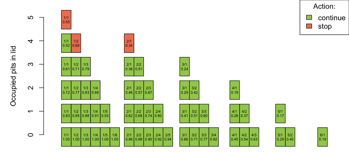
## 20 3 1 1 0  0.22509739     TRUE 0.6125487

One can, e.g., compare the results with the numbers in Fig. 4 of Jehn (2021). The optimal strategy for a two player game is thus to continue as long as only three pits are filled. If four slots are filled, one would only continue, if the situation is 4/1/1. If 5 pits are filled, one should always stop (if possible). The figure below illustrates the strategy for all \(l=0\) states graphically: the y-axis gives \(i\), whereas the label of each box is \(j/k\) followed by the expected probability (with just 2 decimals) to win from this state:

Probability to Win as Start-Player

One surprising finding from the simulations in How to Win a Game (or More) of Super Six was that the start player had a big winning advantage. We use the above algorithm to analytically calculate the probability that the starting players wins the game in a situation where each player initially has 4 sticks.

To compute the winning probability we need to keep in mind that in round 1 we have the additional restriction that only one throw of the dice is allowed for each player. As a consequence, we need to treat the outcome of round 1 separately. There are four possible states that Player 1 starts from in round 2:

1. Both players throw a 6 (\(p=\frac{1}{36}\)) in round 1; round 2 continues from state \(0/3/3/1\)
2. One of the players (but not both!) throws a six (\(p=\frac{10}{36}\)), round 2 continues from state \(1/3/3/1\)
3. Both sticks from round 1 end up in the lid (\(p=\frac{5}{6}\frac{4}{6}=\frac{20}{36}\)); round 2 continues from state \(2/3/3/1\)
4. Player 1 throws anything but a 6 and Player 2 throws the same (\(p=\frac{5}{6}\frac{1}{6}=\frac{5}{36}\)); round 2 continues from state \(0/3/5/1\)

We can thus calculate the probability to win as start player in a 4-stick game (assuming both players follow the optimal winning strategy) as

\[ \frac{1}{36} p_{\text{win}}^{\pi^*}(0/3/3/1) + \frac{10}{36} p_{\text{win}}^{\pi^*}(1/3/3/1) + \frac{20}{36} p_{\text{win}}^{\pi^*}(2/3/3/1) + \frac{5}{36} p_{\text{win}}^{\pi^*}(0/3/5/1). \] We compute this in R with reticulate calls to the Python function calculating the winning probability for a given state:

# States and their probabilities after round 1
round2 <- tibble(
  state = list(c(0,3,3,1), c(1,3,3,1), c(2,3,3,1), c(0,3,5,1)),
  prob = c(1, 10, 20, 5) / 36
)

# Compute the probability to win from round 2 on for a given state
p_win <- function(s) {
  py$optimal_strategy(as.integer(sum(s))) %>% 
             filter( i == s[1] &  j == s[2] &  
                     k == s[3] &  l == s[4]) %>% 
             pull(prob)
} 

# Compute winning probabilities for each state and do the weighted
# sum to get the overall probability to win as start player
(res <- round2 %>% 
  rowwise() %>% 
  mutate(p_win = p_win(state)) %>% 
  ungroup() %>% 
  #unnest_wider(col=state, names_sep=".") %>% 
  summarise(p_win = sum(prob*p_win)))

## # A tibble: 1 × 1
##   p_win
##   <dbl>
## 1 0.602

This corroborates the previous finding that the start player has a 60% probability to win the game when both players play the optimal strategy.

Discussion

Dynamic programming is an important foundation for reinforcement learning. We can use it to find optimal strategies in fully observable stochastic environments. For environments with reasonable sized state spaces and with a known stochastic model for the transitions between states, dynamic programming is a direct method to get exact solutions. No complex approximate solutions, as e.g. discussed in Part 2 of Sutton and Barto (2020), are needed.

Appendix: Python code

The Python code for value iteration can be found as value_iteration.py.

# Python implementation of value iteration to find the optimal strategy in Super Six  
#
# Author: Michael Höhle
# Date:   2023-03-16
#
# Semi-manual translation of the R code in value_iteration.R to python with the 
# help of OpenAI's text-davinci-003 API playground feature https://platform.openai.com/playground/p/default-text-to-command?model=text-davinci-003.

import numpy as np
import pandas as pd

def make_situations(n):
    """Returns all situations in a game with n sticks left

    Parameters
    ----------
    n : int
        The number of sticks left in the game
    
    Returns
    -------
    list
        a list of with entries [i,j,k] 
    """
    res = []
    # Number of sticks in the lid
    for i in range(min(n,5),-1,-1):
        # Number of sticks of player 1
        for j in range(n,0,-1):
            # Number of sticks of player 2
            k = n - i - j
            # Only add valid states
            if (i>=0  and not (j<=0 or k<=0)):
                # Append the state as an array [i,j,k]
                res.append([i,j,k])
    return(res)


def make_states(n):
    """All states when there are n sticks in the game left

    We distinguish between states with a choice if to throw the dice and those without

    Parameters
    ----------
    n : int
        The number of sticks left in the game
    
    Returns
    -------
    list
        a list of with entries [i,j,k] 
    """   
    states = []
    for i in range(1,n+1):
        s = make_situations(i)
        # Make list comprehension which adds a fourth component indicating if the move is forced (0=no, 1=yes)
        for j in range(2):
            states.extend([x + [j] for x in s])
    # Sort the list
    states.sort(reverse=True)
    return(states)

def swap(state, forced_move = None):
    """
    Swap the number of sticks of player 1 and 2

    Parameters
    ----------
    state : vector of length 4
        The state of the game as a vector with 4 components

    forced_move : bool
        If the move is forced (i.e. the player has to swap the sticks)

    Returns
    -------
        The new state as a vector of length 4
    """
    res = [state[0], state[2], state[1], state[3]]
    if (forced_move != None):
        res[3] = forced_move
    return(res)

def add_state(state, Delta, forced_move = None):
    res = [sum(x) for x in zip(state, Delta)]
    if (forced_move != None):
        res[3] = forced_move
    return(res)


def R(state):
    """The immediate reward function
    
    Parameters
    ----------
    state : list
        The state of the game as a vector with 4 components
        
    Returns
    -------
    double The reward R(state), i.e. 1 if player 1 wins, -1 if player 2 wins, 0 otherwise
        
    """
    # A terminal state (player 1 = 0)
    if state[1] == 0:
        return 1
    # A terminal state (player 2 = 0)
    if state[2] == 0:
        return -1
    # Other state (nothing)
    return 0

def optimal_strategy(n, debug=False):
    """"Find the optimal strategy for a game with n sticks left
    """

    # Define local variables for the function
    states = make_states(n)
    n_states = len(states)
    ## Storage of the value function
    U_vec = np.zeros(n_states)
    U_vec_prime = np.zeros(n_states)
    ## Storage of the policy/strategy
    pi = np.full(n_states, np.nan)

    # Future reward function.
    # Note terminating states (i=0 or j=0) have zero future reward.
    # The function uses a local variable states and the value function uvec. Might want to add this to the arguments
    def U(state):
        # Terminal state (no future returns)
        if (state[1] == 0):
            return 0
        if (state[2] == 0):
            return 0
        # Find index of the element matching in states vector
        idx = states.index(state)
        # Return value function of the state
        return U_vec[idx]

    ## Loop controls
    stop = False
    epsilon = 1e-10
    iter = 0

    # Value iteration 
    while (stop == False):
        iter += 1
        Delta = 0
        for idx in range(n_states):
            # Translate to integer configuration
            state = states[idx]

            # The 4 possible moves

            # Do vector addition of the variable state and [0, -1, 0, 0]
            state_six = add_state(state,  [0, -1, 0, 0], forced_move=False)
            state_free = add_state(state, [1, -1, 0, 0], forced_move=False)       
            state_occupied = swap(add_state(state, [-1, 1, 0, 0], forced_move=True))
            state_swap     = swap(state, forced_move=True)                 
        
            # Number of sticks in the lid
            i = state[0]

            #Q(s, continue)
            qs_continue = (1/6  * (R(state_six)  +  U(state_six))) + \
                        ((5-i)/6 * (R(state_free) +  U(state_free)) if i<5 else 0) + \
                        (i/6     * (R(state_occupied) - U(state_occupied)) if i>0 else 0)

            #Q(s, stop)
            qs_stop = -(R(state_swap) + U(state_swap))

            # Updated value & strategy if there is a choice.
            if (state[3]==0):
                U_vec_prime[idx] = max(qs_continue, qs_stop)
                pi[idx] = qs_continue > qs_stop
            else: #no choice
                U_vec_prime[idx] = qs_continue
                pi[idx] = 1

            # Discrepancy  
            Delta = max(Delta, abs(U_vec[idx] - U_vec_prime[idx]))

        # Update the value function by copying the new values
        # Note: In NumPy, using "=" would only make a reference to the new vector
        # See https://www.geeksforgeeks.org/array-copying-in-python/
        U_vec = U_vec_prime.copy()

        # Continue the value iteration?  
        if (debug):
            print("iter = ", iter, ", Delta =", Delta)  
        stop = (Delta <= epsilon)

    # Make a tibble containing the strategy  
    strategy = pd.DataFrame({'state': states, 'value': U_vec, 'strategy': pi, 'prob': 1/2*U_vec+1/2})  
    # Split state column into 4 separate columns
    strategy[['i','j','k','l']] = pd.DataFrame(strategy.state.tolist(), index= strategy.index) 
    # Drop the state column
    strategy = strategy.drop(columns=['state'])
    # Convert strategy to boolean
    strategy['strategy'] = strategy['strategy'].astype(bool)
    # Change the order such that the i,j,k,forced_move columns are shown first
    cols = strategy.columns.tolist()
    cols = cols[-4:] + cols[:-4]
    strategy = strategy[cols]

    return(strategy)


#Test function
#make_situations(6)

# Find optimal strategy for game with 6 sticks left
s_best = optimal_strategy(7)
# Print full strategy without row number, https://stackoverflow.com/questions/52396477/printing-a-pandas-dataframe-without-row-number-index
# pd.set_option('display.max_rows', None)
# print(s_best.to_string(index=False))

References